Simulation input configuration

Jump to Detailed configuration structure for an immediate overview of all configuration parameters.

General notes

TORAX’s configuration system allows for fine-grained control over various aspects of the simulation. This configuration can be represented as a nested dictionary, where the top level keys are:

profile_conditions: Configures boundary conditions, initial conditions, and prescribed time-dependence of temperature, density, and current.
numerics: Configures time stepping settings and numerical parameters.
plasma_composition: Configures the distribution of ion species.
geometry: Configures geometry setup and constructs the Geometry object.
pedestal: Configures the pedestal for the simulation.
sources: Selects and configures parameters of the various heat source, particle source, and non-inductive current models.
solver: Selects and configures the PDE solver.
transport: Selects and configures the transport model, and constructs the TransportModel object.
mhd: Selects and configures the MHD models. Currently only a sawtooth model is implemented.
time_step_calculator: Selects the method used to calculate the timestep dt.
restart: Configures optional restart behavior of the simulation.

This configuration dictionary is converted internally to a Pydantic torax.ToraxConfig model via torax.ToraxConfig.from_dict(config_dict).

Configuration dictionaries are typically defined in a Python file, and used via:

run_torax --config='path/to/config.py'

The file `config.py` must have the config dictionary defined as a global variable named CONFIG. See examples/iterhybrid_rampup.py for an example.

See TORAX code structure for more information on TORAX simulation objects. Further details on the internals of the configuration dictionary are found in Detailed configuration structure.

For various definitions, see Glossary of Terms.

Time-dependence and parameter interpolation

Some TORAX parameters are allowed to vary over time, and are labelled with time-varying-scalar and time-varying-array in Detailed configuration structure below.

Time-varying scalars

The following inputs are valid for time-varying-scalar parameters:

A scalar (integer, float, or boolean). The parameter is then not time-dependent.
A time-series dict with {time: value} pairs.
A tuple (time_array, value_array), where time_array is a 1D array of times, and value_array is a 1D array of values of equal length. The 1D arrays can be a NumPy arrays, lists or tuples.
A xarray.DataArray of the form xarray.DataArray(data=value_array, coords={'time': time_array}).

Note that times do not need to be sorted in order of time. Ordering is carried out internally.

For each evaluation of the TORAX solver (PDE solver), time-dependent variables are interpolated at both time \(t\) and time \(t+dt\).

interpolation methods

Currently, two interpolation modes are supported:

'PIECEWISE_LINEAR': linear interpolation of the input time-series (default).
'STEP': stepwise change in values following each traversal above a time value in the time-series.

The interpolation method can be specified by giving a tuple of the form (inputs, interpolation_mode), where inputs is one of the input specifications listed in the previous section. Specifying no interpolation mode is equivalent to (inputs, 'PIECEWISE_LINEAR').

Examples

1. Define a time-dependent total current \(Ip_{tot}\) with piecewise linear interpolation, from \(t=10\) to \(t=100\). \(Ip_{tot}\) rises from 2MA to 15MA, and then stays flat due to constant extrapolation beyond the last time value.

Ip = ({10: 2.0e6, 100: 15.0e6}, 'PIECEWISE_LINEAR')

or more simply, taking advantage of the default.

Ip = {10: 2.0e6, 100: 15.0e6}

2. Define a time-dependent internal boundary condition for ion temperature, T_i_ped, with stepwise changes, starting at \(1~keV\) at \(t=2s\), transitioning to \(3~keV\) at \(t=8s\), and back down to \(1~keV\) at \(t=20s\):

T_i_ped= ({2: 1.0, 8: 3.0, 20: 1.0}, 'STEP')

Time-varying arrays

Parameters marked as time-varying-array are interpolated on a grid (\(t\), \(\hat{\rho}\)). For each time point, an array of values is defined on the spatial \(\hat{\rho}\) grid.

time-varying-array parameters can be defined using either a nested dictionary, or in the form of arrays (represented as a xarray.DataArray object or a tuple of arrays).

Note: \(\hat{\rho}\) is normalized and will take values between 0 and 1.

In the case of non-evolving (prescribed) parameters for each evaluation of the TORAX solver (PDE solver), time-dependent variables are interpolated first along the \(\hat{\rho}\) axis at the cell grid centers and then linearly interpolated in time at both time \(t\) and time \(t+dt\).

For \(t\) greater than or less than the largest or smallest defined time then the interpolation scheme will be applied from the closest time value.

Using a nested dictionary

This is of the form:

{time_1: {rho_11: value_11, rho_12: value_12, ...}, time_2: ...}

At each time_i, we have a radial profile composed of {rho: value} pairs. The ordering of the dict does not matter.

Shortcuts:

Passing a single float value is interpreted as defining a constant profile for all times. For example T_i: 6.0 would be equivalent to passing in T_i: {0.0: {0.0: 6.0}}.
Passing a single dict (instead of dict of dicts) is a shortcut for defining the rho profile for \(t=0.0\). For example, T_i: {0.0: 18.0, 0.95: 5.0, 1.0: 0.2} is a shortcut for T_i: {0.0: {0: 18.0, 0.95: 5.0, 1.0: 0.2}} where \(t=0.0\) is arbitrary (due to constant extrapolation for any input \(t=0.0\)).

Examples:

1. Define an initial profile (at \(t=0.0\)) for \(T_{i}\) with a pedestal.

T_i = {0.0: {0.0: 15.0, 0.95: 3.0, 1.0: 1.0}}

Note: due to constant extrapolation, the t=0.0 here is an arbitrary number and could be anything.

2. Define a time-dependent \(T_{i}\) profile initialised with a pedestal and, if the ion equation is not being evolved by the PDE, to have a prescribed time evolution which decays to a constant \(T_{i}=1\) by \(t=80.0\).

T_i = {0.0: {0.0: 15.0, 0.95: 3.0, 1.0: 1.0}, 80: 1.0}

Using arrays

This can be a tuple of arrays (time_array, rho_norm_array, values_array), or equivalently an xarray.DataArray object of the form:

xarray.DataArray(
  data=values_array,
  coords={'time': time_array, 'rho_norm': rho_norm_array}
)

All arrays can be represented as NumPy arrays or lists.

time_array is a 1D array of times.
values_array is a 2D array of shape (len(time_array), num_values).
rho_norm_array either a 1D array of shape (num_values,), or a 2D array of shape (len(time_array), num_values).

Shortcuts:

(rho_norm_array, values_array): constant in time profile, useful for defining an initial condition or a constant profile. Note that both arrays are now 1D arrays.

Specifying interpolation methods

By default, piecewise linear interpolation is used to interpolate values both in time and in \(\hat{\rho}\). To specify a different interpolation method:

(time_varying_array_value, {'time_interpolation_mode': 'STEP',
'rho_interpolation_mode': 'PIECEWISE_LINEAR'})

where time_varying_array_value is any of the above inputs (nested dictionary, arrays, etc.).

Currently two interpolation modes are supported as for time-varying-scalar:

'PIECEWISE_LINEAR': linear interpolation of the input time-series (default).
'STEP': stepwise change in values following each traversal above a time value in the time-series.

Detailed configuration structure

Data types and default values are written in parentheses. Any declared parameter in a run-specific config, overrides the default value.

Profile conditions

Configures boundary conditions, initial conditions, and (optionally) prescribed time-dependence of temperature, density, and current.

Ip (time-varying-scalar [default = 15.0e6])

Total plasma current in A. Note that if Ip_from_parameters=False in geometry, then this Ip will be overwritten by values from the geometry data. Boundary condition for the \(\psi\) equation if use_v_loop_lcfs_boundary_condition is False. If use_v_loop_lcfs_boundary_condition is True, only used as an initial condition.

use_v_loop_lcfs_boundary_condition (bool = False)

Boundary condition at LCFS for Vloop ( = dpsi_lcfs/dt ). If use_v_loop_lcfs_boundary_condition is True, then the specified Vloop at the LCFS is used to construct the boundary condition for the psi equation; otherwise, Ip is used to construct the boundary condition.

v_loop_lcfs (time-varying-scalar [default = 0.0])

Boundary condition at LCFS for Vloop ( = dpsi_lcfs/dt ). This sets the psi at the next timestep. This is ignored if use_v_loop_lcfs_boundary_condition is False.

T_i_right_bc (time-varying-scalar [default = None])

Temperature boundary condition at r=a_minor. If this is None the boundary condition will instead be taken from T_i at \(\hat{\rho}=1\).

T_e_right_bc (time-varying-scalar [default = None])

Temperature boundary condition at r=a_minor. If this is None the boundary condition will instead be taken from T_e at \(\hat{\rho}=1\).

T_i (time-varying-array [default = {0: {0: 15.0, 1: 1.0}}])

Prescribed or evolving values for ion temperature at different times in units of keV.

T_e (time-varying-array [default = {0: {0: 15.0, 1: 1.0}}])

Prescribed or evolving values for electron temperature at different times in units of keV.

psi (time-varying-array | None [default = None])

Initial values for poloidal flux. If provided, the initial psi will be taken from here. Otherwise, the initial psi will be calculated from either the geometry or the “current_profile_nu formula” dependant on the initial_psi_from_j field.

n_e (time-varying-array [default = {0: {0: 1.2e20, 1: 0.8e20}}])

Prescribed or evolving values for electron density at different times.

If evolve_density==True (see numerics), then time-dependent n_e is ignored, and only the initial value is used.

normalize_n_e_to_nbar (bool = False)

Whether to renormalize the density profile to have the desired line averaged density nbar.

nbar (time-varying-scalar [default = 0.85e20])

Line averaged density. In units of \(m^{-3}\) if n_e_nbar_is_fGW = False. In Greenwald fraction if n_e_nbar_is_fGW = True. \(n_{GW} = I_p/(\pi a^2)\) with a in m, \(n_{GW}\) in \(10^{20} m^{-3}\), Ip in MA.

n_e_nbar_is_fGW (bool = False)

Toggle units of nbar.

n_e_right_bc (time-varying-scalar | None [default = None])

Density boundary condition for r=a_minor. In units of m^-3 if n_e_right_bc_is_fGW = False. In Greenwald fraction if n_e_right_bc_is_fGW = True. If n_e_right_bc is None then the boundary condition will instead be taken from n_e at \(\hat{\rho}=1\).

n_e_right_bc_is_fGW (bool [default = False])

Toggle units of n_e_right_bc.

current_profile_nu (float [default = 1.0])

Peaking factor of initial current, either total or “Ohmic”: \(j = j_0(1 - r^2/a^2)^{\text{current_profile_nu}}\). Used if initial_psi_from_j is True. In that case, then this sets the peaking factor of either the total or Ohmic initial current profile, depending on the initial_j_is_total_current flag.

initial_j_is_total_current (bool [default = False])

Toggle if the initial current formula set by current_profile_nu is the total current, or the Ohmic current. If Ohmic current, then the magnitude of the Ohmic current is set such that the initial total non-inductive current + total Ohmic current equals Ip

initial_psi_from_j (bool [default = False])

Toggles if the initial psi calculation is based on the “current_profile_nu” current formula, or from the psi available in the numerical geometry file. This setting is ignored for the ad-hoc circular geometry, which has no numerical geometry.

numerics

Configures simulation control such as time settings and timestep calculation, equations being solved, constant numerical variables.

t_initial (float [default = 0.0]): Simulation start time, in units of seconds.
t_final (float [default = 5.0]): Simulation end time, in units of seconds.
exact_t_final (bool [default = True]): If True, ensures that the simulation end time is exactly t_final, by adapting the final dt to match.
max_dt (float [default = 2.0]): Maximum size of timesteps allowed in the simulation. This is only used with the chi_time_step_calculator time_step_calculator.
min_dt (float [default = 1e-8]): Minimum timestep allowed in simulation.
chi_timestep_prefactor (float [default = 50.0]): Prefactor in front of chi_timestep_calculator base timestep \(dt_{base}=\frac{dx^2}{2\chi}\) (see time_step_calculator).
fixed_dt (float [default = 1e-1]): Timestep used for fixed_time_step_calculator (see time_step_calculator).
adaptive_dt (bool [default = True]): If True, then if a nonlinear solver does not converge for a given timestep, then dt-backtracking is applied and a new Solver call is made where the timestep is reduced by a factor of dt_reduction_factor. This is applied iteratively until either the solver converges, or min_dt is reached.
dt_reduction_factor (float [default = 3.0]): Used only if adaptive_dt is True. Factor by which the timestep is reduced if a nonlinear solver does not converge for a given timestep.
evolve_ion_heat (bool [default = True]): Solve the ion heat equation in the time-dependent PDE.
evolve_electron_heat (bool [default = True]): Solve the electron heat equation in the time-dependent PDE.
evolve_current (bool [default = False]): Solve the current diffusion equation (evolving \(\psi\)) in the time-dependent PDE.
evolve_density (bool [default = False]): Solve the electron density equation in the time-dependent PDE.
resistivity_multiplier (time-varying-scalar [default = 1.0]): 1/multiplication factor for \(\sigma\) (conductivity) to reduce the current diffusion timescale to be closer to the energy confinement timescale, for testing purposes.
adaptive_T_source_prefactor (float [default = 1e10]): Prefactor for adaptive source term for setting temperature internal boundary conditions.
adaptive_n_source_prefactor (float [default = 1e8]): Prefactor for adaptive source term for setting density internal boundary conditions.

plasma_composition

Defines the distribution of ion species. The keys and their meanings are as follows:

main_ion (dict[str, time-varying-scalar] | str [default = {'D': 0.5, 'T': 0.5}]) Specifies the main ion species.

If a string, it represents a single ion species (e.g., 'D' for deuterium, 'T' for tritium, 'H' for hydrogen). See below for the full list of supported ions.

If a dict, it represents a mixture of ion species with given fractions. By mixture, we mean key value pairs of ion symbols and fractional concentrations, which must sum to 1 within a tolerance of 1e-6. The effective mass and charge of the mixture is the weighted average of the species masses and charges. The fractions can be time-dependent, i.e. are time-varying-scalar. The ion mixture API thus supports features such as time varying isotope ratios.

impurity (dict[str, time-varying-scalar] | str [default = 'Ne']): Specifies the impurity species, following the same syntax as main_ion. A single effective impurity species is currently supported, although multiple impurities can still be defined as a mixture.
Z_eff ( time-varying-array [default = 1.0]): Plasma effective charge number, defined as \(Z_{eff}=\sum_i Z_i^2 \hat{n}_i\), where \(\hat{n}_i\) is the normalized ion density \(n_i/n_e\). For a given \(Z_{eff}\) and impurity charge states, a consistent \(\hat{n}_i\) is calculated, with the appropriate degree of main ion dilution.
Z_i_override (time-varying-scalar | None [default = None]): An optional override for the main ion’s charge (Z) or average charge of an ion mixture. If provided, this value will be used instead of the Z calculated from the main_ion specification.
A_i_override (time-varying-scalar | None [default = None]): An optional override for the main ion’s mass (A) in amu units or average mass of an ion mixture. If provided, this value will be used instead of the A calculated from the main_ion specification.
Z_impurity_override (time-varying-scalar | None [default = None]): As Z_i_override, but for the impurity ion. If provided, this value will be used instead of the Z calculated from the impurity specification.
A_impurity_override (time-varying-scalar | None [default = None]): As A_i_override, but for the impurity ion. If provided, this value will be used instead of the A calculated from the impurity specification.

The average charge state of each ion in each mixture is determined by Mavrin polynomials, which are fitted to atomic data, and in the temperature ranges of interest in the tokamak core, are well approximated as 1D functions of electron temperature. All ions with atomic numbers below Carbon are assumed to be fully ionized.

Plasma composition examples

We remind that for all cases below, the impurity density is solely constrained by the input Z_eff value and the impurity charge state, presently assumed to be fully ionized. Imminent development will support temperature-dependent impurity average charge states,

Pure deuterium plasma:

'plasma_composition': {
    'main_ion': 'D',
    'impurity': 'Ne',  # Neon
    'Z_eff': 1.5,
}

50-50 DT ion mixture:

'plasma_composition': {
    'main_ion': {'D': 0.5, 'T': 0.5},
    'impurity': 'Be',  # Beryllium
    'Z_eff': 1.8,
}

Time-varying DT ion mixture:

'plasma_composition': {
  'main_ion': {
    'D': {0.0: 0.1, 5.0: 0.9},  # D fraction from 0.1 to 0.9
    'T': {0.0: 0.9, 5.0: 0.1},  # T fraction from 0.9 to 0.1
  },
  'impurity': 'W',  # Tungsten
  'Z_eff': 2.0,
}

Allowed ion symbols

The following ion symbols are recognized for main_ion and impurity input fields.

H (Hydrogen)

D (Deuterium)

T (Tritium)

He3 (Helium-3)

He4 (Helium-4)

Li (Lithium)

Be (Beryllium)

C (Carbon)

N (Nitrogen)

O (Oxygen)

Ne (Neon)

Ar (Argon)

Kr (Krypton)

Xe (Xenon)

W (Tungsten)

pedestal

In TORAX we aim to support different models for computing the pedestal width, and electron density, ion temperature and electron temperature at the pedestal top. These models will only be used if the set_pedestal flag is set to True.

model_name (str [default = ‘no_pedestal’]): The model can be configured by setting the model_name key in the pedestal section of the configuration. If this field is not set, then the default model is no_pedestal.
set_pedestal (time-varying-scalar [default = False]): If True use the configured pedestal model to set internal boundary conditions. Do not set internal boundary conditions if False. Internal boundary conditions are set using an adaptive localized source term. While a common use-case is to mock up a pedestal, this feature can also be used for L-mode modeling with a desired internal boundary condition below \(\hat{\rho}=1\).

The following model_name options are currently supported:

no_pedestal

No pedestal profile is set. This is the default option and the equivalent of setting set_pedestal to False.

set_T_ped_n_ped

Directly specify the pedestal width, electron density, ion temperature and electron temperature.

n_e_ped (time-varying-scalar [default = 0.7e20]): Electron density at the pedestal top. In units of reference density if n_e_ped_is_fGW==False. In units of Greenwald fraction if n_e_ped_is_fGW==True.
n_e_ped_is_fGW (time-varying-scalar [default = False]): Toggles units of n_e_ped.
T_i_ped (time-varying-scalar [default = 5.0]): Ion temperature at the pedestal top in units of keV.
T_e_ped (time-varying-scalar [default = 5.0]): Electron temperature at the pedestal top in units of keV.
rho_norm_ped_top (time-varying-scalar [default = 0.91]): Location of pedestal top, in units of \(\hat{\rho}\).

set_P_ped_n_ped

Set the pedestal width, electron density and ion temperature by providing the total pressure at the pedestal and the ratio of ion to electron temperature.

P_ped (time-varying-scalar [default = 10.0]): The plasma pressure at the pedestal in units of \(Pa\).
n_e_ped (time-varying-scalar [default = 0.7]): Electron density at the pedestal top. In units of reference density if n_e_ped_is_fGW==False. In units of Greenwald fraction if n_e_ped_is_fGW==True.
n_e_ped_is_fGW (time-varying-scalar [default = False]): Toggles units of n_e_ped.
T_i_T_e_ratio (time-varying-scalar [default = 1.0]): Ratio of the ion and electron temperature at the pedestal.
rho_norm_ped_top (time-varying-scalar [default = 0.91]): Location of pedestal top, in units of \(\hat{\rho}\).

geometry

geometry_type (str): Geometry model used. A string must be provided from the following options.

'circular'
An ad-hoc circular geometry model. Includes elongation corrections. Not recommended for use apart from for testing purposes.
'chease'
Loads a CHEASE geometry file.
'fbt'
Loads FBT geometry files.
'eqdsk'
Loads a EQDSK geometry file, and carries out the appropriate flux-surface-averages of the 2D poloidal flux. Use of EQDSK geometry comes with the following caveat: The TORAX EQDSK converter has only been tested against CHEASE-generated EQDSK which is COCOS=2. The converter is not guaranteed to work as expected with arbitrary EQDSK input, so please verify carefully. Future work will be done to correctly handle EQDSK inputs provided with a specific COCOS value.

Geometry dicts for all geometry types can contain the following additional keys.

n_rho (int [default = 25]): Number of radial grid points
hires_factor (int [default = 4]): Only used when the initial condition psi is from plasma current. Sets up a higher resolution mesh with nrho_hires = nrho * hi_res_fac, used for j to psi conversions.

Geometry dicts for all non-circular geometry types can contain the following additional keys.

geometry_file (str) See below for information on defaults: Required for CHEASE and EQDSK geometry. Sets the geometry file loaded. The default is set to ‘ITER_hybrid_citrin_equil_cheasedata.mat2cols’ for CHEASE geometry and EQDSK_ITERhybrid_COCOS02.eqdsk` for EQDSK geometry.
geometry_directory (str | None [default = None]): Optionally set the geometry directory. This should be set to an absolute path. If not set, then the default is torax/data/third_party/geo
Ip_from_parameters (bool [default = True]): Toggles whether total plasma current is read from the configuration file, or from the geometry file. If True, then the \(\psi\) calculated from the geometry file is scaled to match the desired \(I_p\).

Geometry dicts for analytical circular geometry require the following additional keys.

R_major (float [default = 6.2]): Major radius “R” in meters.
a_minor (float [default = 2.0]): Minor radius “a” in meters.
B_0 (float [default = 5.3]): Vacuum toroidal magnetic field on axis in \(T\).
elongation_LCFS (float [default = 1.72]): Sets the plasma elongation used for volume, area and q-profile corrections.

Geometry dicts for CHEASE geometry require the following additional keys for denormalization.

R_major (float [default = 6.2]): Major radius “R” in meters.
a_minor (float [default = 2.0]): Minor radius “a” in meters.
B_0 (float [default = 5.3]): Vacuum toroidal magnetic field on axis \(T\).

Geometry dicts for FBT geometry require the following additional keys.

LY_object (dict[str, np.ndarray | float] | str | None [default = None]): Sets a single-slice FBT LY geometry file to be loaded, or alternatively a dict directly containing a single time slice of LY data.
LY_bundle_object (dict[str, np.ndarray | float] | str | None: [default = None]) Sets the FBT LY bundle file to be loaded, corresponding to multiple time-slices, or alternatively a dict directly containing all time-slices of LY data.
LY_to_torax_times (ndarray | None [default = None]): Sets the TORAX simulation times corresponding to the individual slices in the FBT LY bundle file. If not provided, then the times are taken from the LY_bundle_file itself. The length of the array must match the number of slices in the bundle.
L_object (dict[str, np.ndarray | float] | str | None [default = None]): Sets the FBT L geometry file loaded, or alternatively a dict directly containing the L data.

Geometry dicts for EQDSK geometry can contain the following additional keys. It is only recommended to change the default values if issues arise.

n_surfaces (int [default = 100]): Number of surfaces for which flux surface averages are calculated.
last_surface_factor (float [default = 0.99]): Multiplication factor of the boundary poloidal flux, used for the contour defining geometry terms at the LCFS on the TORAX grid. Needed to avoid divergent integrations in diverted geometries.

For setting up time-dependent geometry, a subset of varying geometry parameters and input files can be defined in a geometry_configs dict, which is a time-series of {time: {configs}} pairs. For example, a time-dependent geometry input with 3 time-slices of single-time-slice FBT geometries can be set up as:

'geometry': {
    'geometry_type': 'fbt',
    'Ip_from_parameters': True,
    'geometry_configs': {
        20.0: {
            'LY_file': 'LY_early_rampup.mat',
            'L_file': 'L_early_rampup.mat',
        },
        50.0: {
            'LY_file': 'LY_mid_rampup.mat',
            'L_file': 'L_mid_rampup.mat',
        },
        100.0: {
            'LY_file': 'LY_endof_rampup.mat',
            'L_file': 'L_endof_rampup.mat',
        },
    },
},

Alternatively, for FBT data specifically, TORAX supports loading a bundle of LY files packaged within a single .mat file using LIUQE meqlpack. This eliminates the need to specify multiple individual LY files in the geometry_configs parameter.

To use this feature, set LY_bundle_object to the corresponding .mat file containing the LY bundle. Optionally set LY_to_torax_times as a NumPy array corresponding to times of the individual LY slices within the bundle. If not provided, then the times are taken from the bundle file itself.

Note that LY_bundle_object cannot coexist with LY_file or geometry_configs in the same configuration, and will raise an error if so.

All file loading and geometry processing is done upon simulation initialization. The geometry inputs into the TORAX PDE coefficients are then time-interpolated on-the-fly onto the TORAX time slices where the PDE calculations are done.

transport

Select and configure various transport models. The dictionary consists of keys common to all transport models, and additional keys pertaining to a specific transport model.

model_name (str [default = ‘constant’]): Select the transport model according to the following options:

'constant' Constant transport coefficients.
'CGM' Critical Gradient Model.
'bohm-gyrobohm' Bohm-GyroBohm model.
'qlknn' A QuaLiKiz Neural Network surrogate model, the default is QLKNN_7_11.
'qualikiz' The QuaLiKiz quasilinear gyrokinetic transport model.
'combined' An additive transport model, where contributions from a list of component models are summed to produce a combined total.

rho_min (float [default = 0.0]): \(\hat{\rho}\) above which the transport model is applied. For rho_min > 0, the model will be active in the range rho_min < rho <= rho_max. For rho_min == 0, it will be active in the range rho_min <= rho <= rho_max.
rho_max (float [default = 1.0]): \(\hat{\rho}\) below which the transport model is applied. See comment about rho_min for more detail.
chi_min (float [default = 0.05]): Lower allowed bound for heat conductivities \(\chi\), in units of \(m^2/s\).
chi_max (float [default = 100.0]): Upper allowed bound for heat conductivities \(\chi\), in units of \(m^2/s\).
D_e_min (float [default = 0.05]): Lower allowed bound for particle diffusivity \(D\), in units of \(m^2/s\).
D_e_max (float [default = 100.0]): Upper allowed bound for particle conductivity \(D\), in units of \(m^2/s\).
V_e_min (float [default = -50.0]): Lower allowed bound for particle convection \(V\), in units of \(m^2/s\).
V_e_max (float [default = 50.0]): Upper allowed bound for particle convection \(V\), in units of \(m^2/s\).
smoothing_width (float [default = 0.0]): Width of HWHM Gaussian smoothing kernel operating on transport model outputs. If using the QLKNN_7_11 transport model, the default is set to 0.1.
smooth_everywhere (bool [default = False]): Smooth across entire radial domain regardless of inner and outer patches.
apply_inner_patch (time-varying-scalar [default = False]): If True, set a patch for inner core transport coefficients below rho_inner. Typically used as an ad-hoc measure for MHD (e.g. sawteeth) or EM (e.g. KBM) transport in the inner-core. If using a CombinedTransportModel, ensure that the inner patch is only set on the global model rather than its component models to avoid conflicts.
D_e_inner (time-varying-scalar [default = 0.2]): Particle diffusivity value for inner transport patch.
V_e_inner (time-varying-scalar [default = 0.0]): Particle convection value for inner transport patch.
chi_i_inner (time-varying-scalar [default = 1.0]): Ion heat conduction value for inner transport patch.
chi_e_inner (time-varying-scalar [default = 1.0]): Electron heat conduction value for inner transport patch.
rho_inner (float [default = 0.3]): \(\hat{\rho}\) below which inner patch is applied.
apply_outer_patch (time-varying-scalar [default = False]): If True, set a patch for outer core transport coefficients above rho_outer. Useful for the L-mode near-edge region where models like QLKNN10D are not applicable. Only used if set_pedestal==False. If using a CombinedTransportModel, ensure that the outer patch is only set on the global model rather than its component models to avoid conflicts.
D_e_outer (time-varying-scalar [default = 0.2]): Particle diffusivity value for outer transport patch.
V_e_outer (time-varying-scalar [default = 0.0]): Particle convection value for outer transport patch.
chi_i_outer (time-varying-scalar [default = 1.0]): Ion heat conduction value for outer transport patch.
chi_e_outer (time-varying-scalar [default = 1.0]): Electron heat conduction value for outer transport patch.
rho_outer (float [default = 0.9]): \(\hat{\rho}\) above which outer patch is applied.

constant

Runtime parameters for the prescribed transport model. This model can be used to implement constant coefficients (e.g. chi_i = 1.0 for all rho), as well as time-varying prescribed transport profiles of arbitrary form (such as an exponential decay) using the time-varying-array syntax.

chi_i (time-varying-array [default = 1.0]): Ion heat conductivity. In units of \(m^2/s\).
chi_e (time-varying-array [default = 1.0]): Electron heat conductivity. In units of \(m^2/s\).
D_e (time-varying-array [default = 1.0]): Electron particle diffusion. In units of \(m^2/s\).
V_e (time-varying-array [default = -0.33]): Electron particle convection. In units of \(m^2/s\).

CGM

Runtime parameters for the Critical Gradient Model (CGM).

alpha (float [default = 2.0]): Exponent of chi power law: \(\chi \propto (R/L_{Ti} - R/L_{Ti_crit})^\alpha\).
chi_stiff (float [default = 2.0]): Stiffness parameter.
chi_e_i_ratio (time-varying-scalar [default = 2.0]): Ratio of ion to electron heat conductivity. ITG turbulence has values above 1.
chi_D_ratio (time-varying-scalar [default = 5.0]): Ratio of ion heat conductivity to electron particle diffusion.
VR_D_ratio (time-varying-scalar [default = 0.0]): Ratio of major radius \(\times\) electron particle convection to electron particle diffusion. Sets the electron particle convection in the model. Negative values will set a peaked electron density profile in the absence of sources.

Bohm-GyroBohm

Runtime parameters for the Bohm-GyroBohm model.

chi_e_bohm_coeff (time-varying-scalar [default = 8e-5]): Prefactor for Bohm term for electron heat conductivity.
chi_e_gyrobohm_coeff (time-varying-scalar [default = 5e-6]): Prefactor for GyroBohm term for electron heat conductivity.
chi_i_bohm_coeff (time-varying-scalar [default = 8e-5]): Prefactor for Bohm term for ion heat conductivity.
chi_i_gyrobohm_coeff (time-varying-scalar [default = 5e-6]): Prefactor for GyroBohm term for ion heat conductivity.
chi_e_bohm_multiplier (time-varying-scalar [default = 1.0]): Multiplier for Bohm term for electron heat conductivity. Intended for user-friendly default modification.
chi_e_gyrobohm_multiplier (time-varying-scalar [default = 1.0]): Multiplier for GyroBohm term for electron heat conductivity. Intended for user-friendly default modification.
chi_i_bohm_multiplier (time-varying-scalar [default = 1.0]): Multiplier for Bohm term for ion heat conductivity. Intended for user-friendly default modification.
chi_i_gyrobohm_multiplier (time-varying-scalar [default = 1.0]): Multiplier for GyroBohm term for ion heat conductivity. Intended for user-friendly default modification.
D_face_c1 (time-varying-scalar [default = 1.0]): Constant for the electron diffusivity weighting factor.
D_face_c2 (time-varying-scalar [default = 0.3]): Constant for the electron diffusivity weighting factor.
V_face_coeff (time-varying-scalar [default = -0.1]): Proportionality factor between convectivity and diffusivity.

qlknn

Runtime parameters for the QLKNN model. These parameters determine which model to load, as well as model parameters. To determine which model to load, TORAX uses the following logic:

If model_path is provided, then we load the model from this path.
Otherwise, if qlknn_model_name is provided, we load that model from registered models in the fusion_surrogates library.
If qlknn_model_name is not set either, we load the default QLKNN model from fusion_surrogates (currently QLKNN_7_11).

It is recommended to not set qlknn_model_name, or model_path to use the default QLKNN model.

model_path (str [default = ‘’]): Path to the model. Takes precedence over qlknn_model_name.
qlknn_model_name (str [default = ‘’]): Name of the model. Used to select a model from the fusion_surrogates library.
include_ITG (bool [default = True]): If True, include ITG modes in the total fluxes.
include_TEM (bool [default = True]): If True, include TEM modes in the total fluxes.
include_ETG (bool [default = True]): If True, include ETG modes in the total electron heat flux.
ITG_flux_ratio_correction (float [default = 1.0]): Increase the electron heat flux in ITG modes by this factor. If using QLKNN10D, the default is 2.0. It is a proxy for the impact of the upgraded QuaLiKiz collision operator, in place since QLKNN10D was developed.
ETG_correction_factor (float [default = 1.0/3.0]): Correction factor for ETG electron heat flux. https://gitlab.com/qualikiz-group/QuaLiKiz/-/commit/5bcd3161c1b08e0272ab3c9412fec7f9345a2eef
clip_inputs (bool [default = False]): Whether to clip inputs within desired margin of the QLKNN training set boundaries.
clip_margin (float [default = 0.95]): Margin to clip inputs within desired margin of the QLKNN training set boundaries.
collisionality_multiplier (float [default = 1.0]): Collisionality multiplier. If using QLKNN10D, the default is 0.25. It is a proxy for the upgraded collision operator in QuaLiKiz, in place since QLKNN10D was developed.
avoid_big_negative_s (bool [default = True]): If True, modify input magnetic shear such that \(\hat{s} - \alpha_{MHD} > -0.2\) always, to compensate for the lack of slab ITG modes in QuaLiKiz.
q_sawtooth_proxy (bool [default = True]): To avoid un-physical transport barriers, modify the input q-profile and magnetic shear for zones where \(q < 1\), as a proxy for sawteeth. Where \(q<1\), then the \(q\) and \(\hat{s}\) QLKNN inputs are clipped to \(q=1\) and \(\hat{s}=0.1\).
DV_effective (bool [default = False]): If True, use either \(D_{eff}\) or \(V_{eff}\) for particle transport. See Physics models for more details.
An_min (float [default = 0.05]): \(|R/L_{ne}|\) value below which \(V_{eff}\) is used instead of \(D_{eff}\), if DV_effective==True.

qualikiz

Runtime parameters for the QuaLiKiz model.

n_max_runs (int [default = 2]): Frequency of full QuaLiKiz contour solutions. For n_max_runs>1, every n_max_runs-th call will use the full contour integral solution. Other runs will use the previous solution as the initial guess for the Newton solver, which is significantly faster.
n_processes (int [default = 8]): Number of MPI processes to use for QuaLiKiz.
collisionality_multiplier (float [default = 1.0]): Collisionality multiplier for sensitivity analysis.
avoid_big_negative_s (bool [default = True]): If True, modify input magnetic shear such that \(\hat{s} - \alpha_{MHD} > -0.2\) always, to compensate for the lack of slab ITG modes in QuaLiKiz.
smag_alpha_correction (bool [default = True]): If True, reduce input magnetic shear by \(0.5*\alpha_{MHD}\) to capture the main impact of \(\alpha_{MHD}\), which was not itself part of the QLKNN training set.
q_sawtooth_proxy (bool [default = True]): To avoid un-physical transport barriers, modify the input q-profile and magnetic shear for zones where \(q < 1\), as a proxy for sawteeth. Where \(q<1\), then the \(q\) and \(\hat{s}\) QuaLiKiz inputs are clipped to \(q=1\) and \(\hat{s}=0.1\).
DV_effective (bool [default = False]): If True, use either \(D_{eff}\) or \(V_{eff}\) for particle transport. See Physics models for more details.
An_min (float [default = 0.05]): \(|R/L_{ne}|\) value below which \(V_{eff}\) is used instead of \(D_{eff}\), if DV_effective==True.

combined

A combined (additive) model, where the total transport coefficients are calculated by summing contributions from a list of component models. Each component model is active only within its defined radial domain, set using rho_min` and rho_max. These zones can be overlapping or non-overlapping; in regions of overlap, the total transport coefficients are computed by adding the contributions from component models active at those coordinates. Post-processing (clipping and smoothing) is performed on the summed value.

The runtime parameters are as follows.

transport_models (list[dict]): A list containing config dicts for the component transport models.

Warning

TORAX will throw a ValueError if any of the component transport model configs have apply_inner_patch or apply_outer_patch set to True. Patches must be set in the config of the combined model only.

Example:

'transport': {
  'model_name': 'combined',
  'transport_models': [
    {
      'model_name': 'constant',
        'chi_i': 1.0,
        'rho_max': 0.3,
    },
    {
      'model_name': 'constant',
        'chi_i': 2.0,
        'rho_min': 0.2
        'rho_max': 0.5,
    },
    {
      'model_name': 'constant',
        'chi_i': 0.5,
        'rho_min': 0.5
        'rho_max': 1.0,
    },
  ],
}

This would produce a chi_i profile that looks like the following.

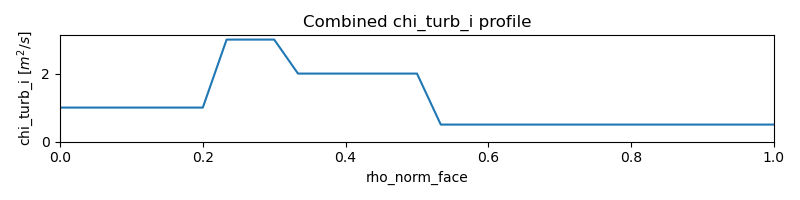
Note that in the region \([0, 0.2]\), only the first component is active, so chi_i = 1.0. In \((0.2, 0.3]\) the first two components are both active, leading to a combined value of chi_i = 3.0. In \((0.3, 0.5]\), only the second model is active (chi_i = 2.0), and in \((0.5, 1.0]\) only the fourth model is active (chi_i = 0.5).

sources

Dictionary with nested dictionaries containing the configurable runtime parameters of all TORAX heat, particle, and current sources. The following runtime parameters are common to all sources, with defaults depending on the specific source. See Physics models For details on the source physics models.

Any source which is not explicitly included in the sources dict, is set to zero. To include a source with default options, the source dict should contain an empty dict. For example, for setting ei_exchange, with default options, as the only active source in sources, set:

'sources': {
    'ei_exchange': {},
}

The configurable runtime parameters of each source are as follows:

prescribed_values (time-varying-array [default = {0: {0: 0, 1: 0}}]): Time varying array of prescribed values for the source. Used if mode is 'PRESCRIBED'.
mode (str [default = ‘zero’]): Defines how the source values are computed. Currently the options are:

'ZERO'
Source is set to zero.
'MODEL'
Source values come from a model in code. Specific model selection where more than one model is available can be done by specifying a model_name. This is documented in the individual source sections.
'PRESCRIBED'
Source values are arbitrarily prescribed by the user. The value is set by prescribed_values, and should be a tuple of values. Each value can contain the same data structures as Time-varying arrays. Note that these values are treated completely independently of each other so for sources with multiple time dimensions, the prescribed values should each contain all the information they need. For sources which affect multiple core profiles, look at the source’s affected_core_profiles property to see the order in which the prescribed values should be provided.

For example, to set ‘fusion_power’ to zero, e.g. for testing or sensitivity purposes, set:

'sources': {
    'fusion': {'mode': 'ZERO'},
}

To set ‘generic_current’ to a prescribed value based on a tuple of numpy arrays, e.g. as defined or loaded from a file in the preamble to the CONFIG dict within config module, set:

'sources': {
    'generic_current': {
        'mode': 'PRESCRIBED',
        'prescribed_values': ((times, rhon, current_profiles),),
    },

where the example times is a 1D numpy array of times, rhon is a 1D numpy array of normalized toroidal flux coordinates, and current_profiles is a 2D numpy array of the current profile at each time. These names are arbitrary, and can be set to anything convenient.

is_explicit (bool [default = False]): Defines whether the source is to be considered explicit or implicit. Explicit sources are calculated based on the simulation state at the beginning of a time step, or do not have any dependance on state. Implicit sources depend on updated states as the iterative solvers evolve the state through the course of a time step. If a source model is complex but evolves over slow timescales compared to the state, it may be beneficial to set it as explicit.

ei_exchange

Ion-electron heat exchange.

mode (str [default = ‘model’])

Qei_multiplier (float [default = 1.0]): Multiplication factor for ion-electron heat exchange term for testing purposes.

bremsstrahlung

Bremsstrahlung model from Wesson, with an optional correction for relativistic effects from Stott PPCF 2005.

mode (str [default = ‘model’])

use_relativistic_correction (bool [default = False])

cyclotron_radiation

Cyclotron radiation model from Albajar NF 2001 with a deposition profile from Artaud NF 2018.

mode (str [default = ‘model’])

wall_reflection_coeff (float [default = 0.9]): Machine-dependent dimensionless parameter corresponding to the fraction of cyclotron radiation reflected off the wall and reabsorbed by the plasma.

beta_min (float [default = 0.5])

beta_max (float [default = 8.0])

beta_grid_size (int [default = 32]): beta in this context is a variable in the temperature profile parameterization used in the Albajar model. The parameter is fit with simple grid search performed over the range [beta_min, beta_max], with beta_grid_size uniformly spaced steps. This parameter must be positive.

ecrh

Electron-cyclotron heating and current drive, based on the local efficiency model in Lin-Liu et al., 2003. Given an EC power density profile and efficiency profile, the model produces the corresponding EC-driven current density profile. The user has three options:

Provide an entire EC power density profile manually (via extra_prescribed_power_density).
Provide the parameters of a Gaussian EC deposition (via gaussian_width, gaussian_location, and P_total).
Any combination of the above.

By default, both the manual and Gaussian profiles are zero. The manual and Gaussian profiles are summed together to produce the final EC deposition profile.

mode (str [default = ‘model’])

extra_prescribed_power_density (time-varying-array [default = {0: {0: 0, 1: 0}}])
EC power density deposition profile, in units of \(W/m^3\).

gaussian_width (time-varying-scalar [default = 0.1])
Width of Gaussian EC power density deposition profile.

gaussian_location (time-varying-scalar [default = 0.0])
Location of Gaussian EC power density deposition profile on the normalized rho grid.

P_total (time-varying-scalar [default = 0.0])
Integral of the Gaussian EC power density profile, setting the total power.

current_drive_efficiency (time-varying-array [default = {0: {0: 0.2, 1: 0.2}}])
Dimensionless local efficiency profile for conversion of EC power to current.

fusion

DT fusion power from the Bosch-Hale parameterization. Uses the D and T fractions from the main_ion ion mixture.

mode (str [default = ‘model’])

gas_puff

Exponential based gas puff source. No first-principle-based model is yet implemented in TORAX.

mode (str [default = ‘model’])

puff_decay_length (time-varying-scalar [default = 0.05]): Gas puff decay length from edge in units of \(\hat{\rho}\).
S_total (time-varying-scalar [default = 1e22]): Total number of particle source in units of particles/s.

generic_current

Generic external current profile, parameterized as a Gaussian.

mode (str [default = ‘model’])

gaussian_location (time-varying-scalar [default = 0.4]): Gaussian center of current profile in units of \(\hat{\rho}\).
gaussian_width (time-varying-scalar [default = 0.05]): Gaussian width of current profile in units of \(\hat{\rho}\).
I_generic (time-varying-scalar [default = 3.0e6]): Total current in A. Only used if use_absolute_current==True.
fraction_of_total_current (time-varying-scalar [default = 0.2]): Sets total generic_current to be a fraction fraction_of_total_current of the total plasma current. Only used if use_absolute_current==False.
use_absolute_current (bool [default = False]): Toggles relative vs absolute external current setting.

generic_heat

A utility source module that allows for a time-dependent Gaussian ion and electron heat source.

mode (str [default = ‘model’])

gaussian_location (time-varying-scalar [default = 0.0]): Gaussian center of source profile in units of \(\hat{\rho}\).
gaussian_width (time-varying-scalar [default = 0.25]): Gaussian width of source profile in units of \(\hat{\rho}\).
P_total (time-varying-scalar [default = 120e6]): Total source power in W. High default based on total ITER power including alphas.
electron_heat_fraction (time-varying-scalar [default = 0.66666]): Electron heating fraction.
absorption_fraction (time-varying-scalar [default = 0.0]): Fraction of input power that is absorbed by the plasma.

generic_particle

Time-dependent Gaussian particle source. No first-principle-based model is yet implemented in TORAX.

mode (str [default = ‘model’])

deposition_location (time-varying-scalar [default = 0.0]): Gaussian center of source profile in units of \(\hat{\rho}\).
particle_width (time-varying-scalar [default = 0.25]): Gaussian width of source profile in units of \(\hat{\rho}\).
S_total (time-varying-scalar [default = 1e22]): Total particle source in units of particles/s.

icrh

Ion cyclotron heating using a surrogate model of the TORIC ICRH spectrum solver simulation https://meetings.aps.org/Meeting/DPP24/Session/NP12.106. This source is currently SPARC specific.

Weights and configuration for the surrogate model are needed to use this source. By default these are expected to be found under '~/toric_surrogate/TORIC_MLP_v1/toricnn.json'. To use a different file path an alternative path can be provided using the TORIC_NN_MODEL_PATH environment variable which should point to a compatible JSON file.

mode (str [default = ‘model’])

model_path (str | None [default = None]): Path to the JSON file containing the weights and configuration for the surrogate model. If None, the default path '~/toric_surrogate/TORIC_MLP_v1/toricnn.json' is used.
wall_inner (float [default = 1.24]): Inner radial location of first wall at plasma midplane level [m].
wall_outer (float [default = 2.43]): Outer radial location of first wall at plasma midplane level [m].
frequency (time-varying-scalar [default = 120e6]): ICRF wave frequency in Hz.
minority_concentration (time-varying-scalar [default = 0.03]): Helium-3 minority fractional concentration relative to the electron density.
P_total (time-varying-scalar [default = 10e6]): Total injected source power in W.

See Physics models for more detail.

impurity_radiation

Various models for impurity radiation. Runtime params for each available model are listed separately

mode (str [default = ‘model’])

model_name (str [default = ‘mavrin_fit’])

The following models are available:

'mavrin_fit'
Polynomial fits to ADAS data from Mavrin, 2018.

radiation_multiplier (float [default = 1.0]). Multiplication factor for radiation term for testing sensitivities.
'P_in_scaled_flat_profile'
Sets impurity radiation to be a constant fraction of the total external input power.

fraction_P_heating (float [default = 1.0]). Fraction of total external input heating power to use for impurity radiation.

ohmic

Ohmic power.

mode (str [default = ‘model’])

pellet

Time-dependent Gaussian pellet source. No first-principle-based model is yet implemented in TORAX.

mode (str [default = ‘model’])

pellet_deposition_location (time-varying-scalar [default = 0.85]): Gaussian center of source profile in units of \(\hat{\rho}\).
pellet_width (time-varying-scalar [default = 0.1]): Gaussian width of source profile in units of \(\hat{\rho}\).
S_total (time-varying-scalar [default = 2e22]): Total particle source in units of particles/s

mhd

Configuration for MHD models. Currently only the sawtooth model is implemented. If the mhd key or the nested sawtooth key is absent or set to None, the sawtooth model will be disabled.

sawtooth

model_name (str [default = ‘simple’]): Currently only ‘simple’ is supported.

simple trigger model parameters:

s_critical (time-varying-scalar [default = 0.1]) The critical magnetic shear value at the q=1 surface. A crash is triggered only if the shear exceeds this value.
minimum_radius (time-varying-scalar [default = 0.05]) The minimum normalized radius (\(\hat{\rho}\)) of the q=1 surface required to trigger a crash.

model_name (str [default = ‘simple’]): Currently only ‘simple’ is supported.

simple redistribution model parameters:

flattening_factor (time-varying-scalar [default = 1.01]): Factor determining the degree of flattening inside the q=1 surface.
mixing_radius_multiplier (time-varying-scalar [default = 1.1]): Multiplier applied to \(\hat{\rho}_{q=1}\) to determine the mixing radius \(\hat{\rho}_{mix}\).

crash_step_duration (float [default = 1e-3]):: Duration of a sawtooth crash step in seconds. This is how much the solver time will be bumped forward during a crash.

solver

Select and configure the Solver object, which evolves the PDE system by one timestep. See TORAX solver details for further details. The dictionary consists of keys common to all solvers. Additional fields for parameters pertaining to a specific solver are defined in the relevant section below.

solver_type (str [default = ‘linear’]): Selected PDE solver algorithm. The current options are:

'linear'
Linear solver where PDE coefficients are set at fixed values of the state. An approximation of the nonlinear solution is optionally carried out with a predictor-corrector method, i.e. fixed point iteration of the PDE coefficients.
'newton_raphson'
Nonlinear solver using the Newton-Raphson iterative algorithm, with backtracking line search, and timestep backtracking, for increased robustness.
'optimizer'
Nonlinear solver using the jaxopt library.

theta_implicit (float [default = 1.0]): theta value in the theta method of time discretization. 0 = explicit, 1 = fully implicit, 0.5 = Crank-Nicolson.
use_predictor_corrector (bool [default = True]): Enables use_predictor_corrector iterations with the linear solver.
n_corrector_steps (int [default = 10]): Number of corrector steps for the predictor-corrector linear solver. 0 means a pure linear solve with no corrector steps. Must be a positive integer.
use_pereverzev (bool [default = False]): Use Pereverzev-Corrigan terms in the heat and particle flux when using the linear solver. Critical for stable calculation of stiff transport, at the cost of introducing non-physical lag during transient. Also used for the linear_step initial guess mode in the nonlinear solvers.
chi_pereverzev (float [default = 30.0]): Large heat conductivity used for the Pereverzev-Corrigan term.
D_pereverzev (float [default = 15.0]): Large particle diffusion used for the Pereverzev-Corrigan term.

linear

No extra parameters are defined for the linear solver.

newton_raphson

log_iterations (bool [default = False]): If True, logs information about the internal state of the Newton-Raphson solver. For the first iteration, this contains the initial residual value and time-step size. For subsequent iterations, this contains the iteration step number, the current value of the residual, and the current value of tau, which is the relative reduction in Newton step size compared to the original Newton step size. If the solver does not converge, then these inner iterations will restart at a smaller timestep size if adaptive_dt=True in the numerics config dict.
initial_guess_mode (str [default = ‘linear_step’]): Sets the approach taken for the initial guess into the Newton-Raphson solver for the first iteration. Two options are available:

x_old
Use the state at the beginning of the timestep.
linear_step
Use the linear solver to obtain an initial guess to warm-start the nonlinear solver. If used, is recommended to do so with the use_predictor_corrector solver and several corrector steps. It is also strongly recommended to use_pereverzev=True if a stiff transport model like qlknn is used.

residual_tol (float [default = 1e-5]): PDE residual magnitude tolerance for successfully exiting the iterative solver.
residual_coarse_tol (float [default = 1e-2]): If the solver hits an exit criterion due to small steps or many iterations, but the residual is still below coarse_tol, then the step is allowed to successfully pass, and a warning is passed to the user.
n_max_iterations (int [default = 30]): Maximum number of allowed Newton iterations. If the number of iterations surpasses maxiter, then the solver will exit in an unconverged state. The step will still be accepted if residual < coarse_tol, otherwise dt backtracking will take place if enabled.
delta_reduction_factor (float [default = 0.5]): Reduction of Newton iteration step size in the backtracking line search. If in a given iteration, the new state is unphysical (e.g. negative temperatures) or the residual increases in magnitude, then a smaller step will be iteratively taken until the above conditions are met.
tau_min (float [default = 0.01]): tau is the relative reduction in step size: delta/delta_original, following backtracking line search, where delta_original is the step in state \(x\) that minimizes the linearized PDE system. If following some iterations, tau < tau_min, then the solver will exit in an unconverged state. The step will still be accepted if residual < coarse_tol, otherwise dt backtracking will take place if enabled.

optimizer

initial_guess_mode (str [default = ‘linear_step’]): Sets the approach taken for the initial guess into the Newton-Raphson solver for the first iteration. Two options are available:

x_old
Use the state at the beginning of the timestep.
linear_step
Use the linear solver to obtain an initial guess to warm-start the nonlinear solver. If used, is recommended to do so with the use_predictor_corrector solver and several corrector steps. It is also strongly recommended to use_pereverzev=True if a stiff transport model like qlknn is used.

loss_tol (float [default = 1e-10]): PDE loss magnitude tolerance for successfully exiting the iterative solver. Note: the default tolerance here is smaller than the default tolerance for the Newton-Raphson solver because it’s a tolerance on the loss (square of the residual).
n_max_iterations (int [default = 100]): Maximum number of allowed optimizer iterations.

time_step_calculator

calculator_type (str [default = ‘chi’]): The name of the time_step_calculator, a method which calculates dt at every timestep. Two methods are currently available:

'fixed'
dt is equal to fixed_dt defined in numerics. If the Newton-Raphson solver is being used and adaptive_dt==True in the numerics config dict, then in practice some steps may have lower dt if the solver needed to backtrack.
'chi'
adaptive dt method, where dt is a multiple of a base dt inspired by the explicit stability limit for parabolic PDEs: \(dt_{base}=\frac{dx^2}{2\chi}\), where \(dx\) is the grid resolution and \(\chi=max(\chi_i, \chi_e)\). dt=chi_timestep_prefactor * dt_base, where chi_timestep_prefactor is defined in numerics, and can be significantly larger than unity for implicit solvers.

Scaling the timestep to be \(\propto \chi\) helps protect against traversing through fast transients, if there is a desire for them to be fully resolved.

tolerance (float [default = 1e-7]): The tolerance within the final time for which the simulation will be considered done.

neoclassical

bootstrap_current

model_name (str [default = ‘sauter’]): The name of the model to use. If not provided, the default is to use the Sauter model with default values. One of sauter or zeros is supported.

If the sauter model is used, the following parameters can be set:

bootstrap_multiplier (float [default = 1.0]): Multiplier for the bootstrap current.

conductivity

model_name (str [default = ‘sauter’]): The name of the Sauter model to use. If not provided, the default is to use the Sauter model with default values.

Additional Notes

What triggers a recompilation?

Most config options can be changed without recompiling the simulation code.

Some define the fundamental structure of the simulation and require JAX recompilation if changed. Examples include the number of grid points or the choice of transport model. A partial list is provided below.

CONFIG['geometry']['nrho']
CONFIG['numerics']['evolve_ion_heat']
CONFIG['numerics']['evolve_electron_heat']
CONFIG['numerics']['evolve_current']
CONFIG['numerics']['evolve_density']
CONFIG['transport']['model_name']
CONFIG['solver']['solver_type']
CONFIG['time_step_calculator']['calculator_type']
CONFIG['sources']['source_name']['is_explicit']
CONFIG['sources']['source_name']['mode']

In the future we aim to provide more transparency at the config level for which configuration options recompilation is required.

Config example

An example configuration dict, corresponding to a non-rigorous demonstration mock-up of a time-dependent ITER hybrid scenario rampup (presently with a fixed CHEASE geometry), is shown below. The configuration file is also available in torax/examples/iterhybrid_rampup.py.

CONFIG = {
    'plasma_composition': {
        'main_ion': {'D': 0.5, 'T': 0.5},
        'impurity': 'Ne',
        'Z_eff': 1.6,
    },
    'profile_conditions': {
        'Ip': {0: 3e6, 80: 10.5e6},
        # initial condition ion temperature for r=0 and r=a_minor
        'T_i': {0.0: {0.0: 6.0, 1.0: 0.1}},
        'T_i_right_bc': 0.1,  # boundary condition ion temp for r=a_minor
        # initial condition electron temperature between r=0 and r=a_minor
        'T_e': {0.0: {0.0: 6.0, 1.0: 0.1}},
        'T_e_right_bc': 0.1,  # boundary condition electron temp for r=a_minor
        'n_e_right_bc_is_fGW': True,
        'n_e_right_bc': {0: 0.1, 80: 0.3},
        'n_e_nbar_is_fGW': True,
        'nbar': 1,
        'n_e': {0: {0.0: 1.5, 1.0: 1.0}},  # Initial electron density profile
        'T_i_ped': 1.0,
        'T_e_ped': 1.0,
        'n_e_ped_is_fGW': True,
        'n_e_ped': {0: 0.3, 80: 0.7},
        'Ped_top': 0.9,
    },
    'numerics': {
        't_final': 80,
        'fixed_dt': 2,
        'evolve_ion_heat': True,
        'evolve_electron_heat': True,
        'evolve_current': True,
        'evolve_density': True,
        'dt_reduction_factor': 3,
        'adaptive_T_source_prefactor': 1.0e10,
        'adaptive_n_source_prefactor': 1.0e8,
    },
    'geometry': {
        'geometry_type': 'chease',
        'geometry_file': 'ITER_hybrid_citrin_equil_cheasedata.mat2cols',
        'Ip_from_parameters': True,
        'R_major': 6.2,
        'a_minor': 2.0,
        'B_0': 5.3,
    },
    'sources': {
        'j_bootstrap': {},
        'generic_current': {
            'fraction_of_total_current': 0.15,
            'gaussian_width': 0.075,
            'gaussian_location': 0.36,
        },
        'pellet': {
            'S_total': 0.0e22,
            'pellet_width': 0.1,
            'pellet_deposition_location': 0.85,
        },
        'generic_heat': {
            'gaussian_location': 0.12741589640723575,
            'gaussian_width': 0.07280908366127758,
            # total heating (with a rough assumption of radiation reduction)
            'P_total': 20.0e6,
            'electron_heat_fraction': 1.0,
        },
        'fusion': {},
        'ei_exchange': {},
    },
    'transport': {
        'model_name': 'qlknn',
        'apply_inner_patch': True,
        'D_e_inner': 0.25,
        'V_e_inner': 0.0,
        'chi_i_inner': 1.5,
        'chi_e_inner': 1.5,
        'rho_inner': 0.3,
        'apply_outer_patch': True,
        'D_e_outer': 0.1,
        'V_e_outer': 0.0,
        'chi_i_outer': 2.0,
        'chi_e_outer': 2.0,
        'rho_outer': 0.9,
        'chi_min': 0.05,
        'chi_max': 100,
        'D_e_min': 0.05,
        'D_e_max': 50,
        'V_e_min': -10,
        'V_e_max': 10,
        'smoothing_width': 0.1,
        'qlknn_params': {
            'DV_effective': True,
            'avoid_big_negative_s': True,
            'An_min': 0.05,
            'ITG_flux_ratio_correction': 1,
        },
    },
    'pedestal': {
        'model_name': 'set_T_ped_n_ped',
        'set_pedestal': True,
        'T_i_ped': 1.0,
        'T_e_ped': 1.0,
        'rho_norm_ped_top': 0.95,
    },
    'solver': {
        'solver_type': 'newton_raphson',
        'use_predictor_corrector': True,
        'n_corrector_steps': 10,
        'chi_pereverzev': 30,
        'D_pereverzev': 15,
        'use_pereverzev': True,
        'log_iterations': False,
    },
    'time_step_calculator': {
        'calculator_type': 'fixed',
    },
}

Restarting a simulation

In order to restart a simulation a field can be added to the config.

For example following a simulation in which a state file is saved to /path/to/torax_state_file.nc, if we want to start a new simulation from the state of the previous one at t=10 we could add the following to our config:

{
    'filename': '/path/to/torax_state_file.nc',
    'time': 10,
    'do_restart': True,  # Toggle to enable/disable a restart.
    # Whether or not to pre"stitch" the contents of the loaded state file up
    # to `time` with the output state file from this simulation.
    'stitch': True,
}

The subsequence simulation will then recreate the state from t=10 in the previous simulation and then run the simulation from that point in time. For all subsequent steps the dynamic runtime parameters will be constructed using the given runtime parameter configuration (from t=10 onwards).

If the requested restart time is not exactly available in the state file, the simulation will restart from the closest available time. A warning will be logged in this case.

We envisage this feature being useful for example to:

restart a(n expensive) simulation that was healthy up till a certain time and then failed. After discovering the issue for breakage you could then restart the sim from the last healthy point.
do uncertainty quantification by sweeping lots of configs following running a simulation up to a certain point in time. After running the initial simulation you could then modify and sweep the runtime parameter config in order to do some uncertainty quantification.