Simulation input configuration

Jump to Detailed configuration structure for an immediate overview of all configuration parameters.

General notes

TORAX’s configuration system allows for fine-grained control over various aspects of the simulation. This configuration can be represented as a nested dictionary, where the top level keys are:

• profile_conditions: Configures boundary conditions, initial conditions, and prescribed time-dependence of temperature, density, and current.

• numerics: Configures time stepping settings and numerical parameters.

• plasma_composition: Configures the distribution of ion species.

• geometry: Configures geometry setup and constructs the Geometry object.

• pedestal: Configures the pedestal for the simulation.

• edge: Selects and configures the edge physics model.

• sources: Selects and configures parameters of the various heat source, particle source, and non-inductive current models.

• solver: Selects and configures the PDE solver.

• transport: Selects and configures the transport model, and constructs the TransportModel object.

• mhd: Selects and configures the MHD models. Currently only a sawtooth model is implemented.

• time_step_calculator: Selects the method used to calculate the timestep dt.

• restart: Configures optional restart behavior of the simulation.

This configuration dictionary is converted internally to a Pydantic torax.ToraxConfig model via torax.ToraxConfig.from_dict(config_dict).

Configuration dictionaries are typically defined in a Python file, and used via:

run_torax --config='path/to/config.py'

The file `config.py` must have the config dictionary defined as a global variable named CONFIG. See examples/iterhybrid_rampup.py for an example.

See TORAX code structure for more information on TORAX simulation objects. Further details on the internals of the configuration dictionary are found in Detailed configuration structure.

For various definitions, see Glossary of Terms.

Time-dependence and parameter interpolation

Some TORAX parameters are allowed to vary over time, and are labelled with time-varying-scalar and time-varying-array in Detailed configuration structure below.

Time-varying scalars

The following inputs are valid for time-varying-scalar parameters:

• A scalar (integer, float, or boolean). The parameter is then not time-dependent.

• A time-series dict with {time: value} pairs.

• A tuple (time_array, value_array), where time_array is a 1D array of times, and value_array is a 1D array of values of equal length. The 1D arrays can be a NumPy arrays, lists or tuples.

• A xarray.DataArray of the form xarray.DataArray(data=value_array, coords={'time': time_array}).

Note that times do not need to be sorted in order of time. Ordering is carried out internally.

For each evaluation of the TORAX solver (PDE solver), time-dependent variables are interpolated at both time \(t\) and time \(t+dt\).

interpolation methods

Currently, two interpolation modes are supported:

• 'PIECEWISE_LINEAR': linear interpolation of the input time-series (default).

• 'STEP': stepwise change in values following each traversal above a time value in the time-series.

The interpolation method can be specified by giving a tuple of the form (inputs, interpolation_mode), where inputs is one of the input specifications listed in the previous section. Specifying no interpolation mode is equivalent to (inputs, 'PIECEWISE_LINEAR').

Examples

1. Define a time-dependent total current \(Ip_{tot}\) with piecewise linear interpolation, from \(t=10\) to \(t=100\). \(Ip_{tot}\) rises from 2MA to 15MA, and then stays flat due to constant extrapolation beyond the last time value.

Ip = ({10: 2.0e6, 100: 15.0e6}, 'PIECEWISE_LINEAR')

or more simply, taking advantage of the default.

Ip = {10: 2.0e6, 100: 15.0e6}

2. Define a time-dependent internal boundary condition for ion temperature, T_i_ped, with stepwise changes, starting at \(1~keV\) at \(t=2s\), transitioning to \(3~keV\) at \(t=8s\), and back down to \(1~keV\) at \(t=20s\):

T_i_ped= ({2: 1.0, 8: 3.0, 20: 1.0}, 'STEP')

Time-varying arrays

Parameters marked as time-varying-array are interpolated on a grid (\(t\), \(\hat{\rho}\)). For each time point, an array of values is defined on the spatial \(\hat{\rho}\) grid.

time-varying-array parameters can be defined using either a nested dictionary, or in the form of arrays (represented as a xarray.DataArray object or a tuple of arrays).

Note: \(\hat{\rho}\) is normalized and will take values between 0 and 1.

In the case of non-evolving (prescribed) parameters for each evaluation of the TORAX solver (PDE solver), time-dependent variables are interpolated first along the \(\hat{\rho}\) axis at the cell grid centers and then linearly interpolated in time at both time \(t\) and time \(t+dt\).

For \(t\) greater than or less than the largest or smallest defined time then the interpolation scheme will be applied from the closest time value.

Using a nested dictionary

This is of the form:

{time_1: {rho_11: value_11, rho_12: value_12, ...}, time_2: ...}

At each time_i, we have a radial profile composed of {rho: value} pairs. The ordering of the dict does not matter.

Shortcuts:

• Passing a single float value is interpreted as defining a constant profile for all times. For example T_i: 6.0 would be equivalent to passing in T_i: {0.0: {0.0: 6.0}}.

• Passing a single dict (instead of dict of dicts) is a shortcut for defining the rho profile for \(t=0.0\). For example, T_i: {0.0: 18.0, 0.95: 5.0, 1.0: 0.2} is a shortcut for T_i: {0.0: {0: 18.0, 0.95: 5.0, 1.0: 0.2}} where \(t=0.0\) is arbitrary (due to constant extrapolation for any input \(t=0.0\)).

Examples:

1. Define an initial profile (at \(t=0.0\)) for \(T_{i}\) with a pedestal.

T_i = {0.0: {0.0: 15.0, 0.95: 3.0, 1.0: 1.0}}

Note: due to constant extrapolation, the t=0.0 here is an arbitrary number and could be anything.

2. Define a time-dependent \(T_{i}\) profile initialised with a pedestal and, if the ion equation is not being evolved by the PDE, to have a prescribed time evolution which decays to a constant \(T_{i}=1\) by \(t=80.0\).

T_i = {0.0: {0.0: 15.0, 0.95: 3.0, 1.0: 1.0}, 80: 1.0}

Using arrays

This can be a tuple of arrays (time_array, rho_norm_array, values_array), or equivalently an xarray.DataArray object of the form:

xarray.DataArray(
  data=values_array,
  coords={'time': time_array, 'rho_norm': rho_norm_array}
)

All arrays can be represented as NumPy arrays or lists.

• time_array is a 1D array of times.

• values_array is a 2D array of shape (len(time_array), num_values).

• rho_norm_array either a 1D array of shape (num_values,), or a 2D array of shape (len(time_array), num_values).

Shortcuts:

• (rho_norm_array, values_array): constant in time profile, useful for defining an initial condition or a constant profile. Note that both arrays are now 1D arrays.

Specifying interpolation methods

By default, piecewise linear interpolation is used to interpolate values both in time and in \(\hat{\rho}\). To specify a different interpolation method:

(time_varying_array_value, {'time_interpolation_mode': 'STEP',
'rho_interpolation_mode': 'PIECEWISE_LINEAR'})

where time_varying_array_value is any of the above inputs (nested dictionary, arrays, etc.).

Currently two interpolation modes are supported as for time-varying-scalar:

• 'PIECEWISE_LINEAR': linear interpolation of the input time-series (default).

• 'STEP': stepwise change in values following each traversal above a time value in the time-series.

Detailed configuration structure

Data types and default values are written in parentheses. Any declared parameter in a run-specific config, overrides the default value.

Profile conditions

Configures boundary conditions, initial conditions, and (optionally) prescribed time-dependence of temperature, density, and current.

Ip (time-varying-scalar [default = 15.0e6])

Total plasma current in A. Note that if Ip_from_parameters=False in geometry, then this Ip will be overwritten by values from the geometry data. Boundary condition for the \(\psi\) equation if use_v_loop_lcfs_boundary_condition is False. If use_v_loop_lcfs_boundary_condition is True, only used as an initial condition.

use_v_loop_lcfs_boundary_condition (bool = False)

Boundary condition at LCFS for Vloop ( = dpsi_lcfs/dt ). If use_v_loop_lcfs_boundary_condition is True, then the specified Vloop at the LCFS is used to construct the boundary condition for the psi equation; otherwise, Ip is used to construct the boundary condition.

v_loop_lcfs (time-varying-scalar [default = 0.0])

Boundary condition at LCFS for Vloop ( = dpsi_lcfs/dt ). This sets the psi at the next timestep. This is ignored if use_v_loop_lcfs_boundary_condition is False.

T_i_right_bc (time-varying-scalar [default = None])

Temperature boundary condition at r=a_minor. If this is None the boundary condition will instead be taken from T_i at \(\hat{\rho}=1\). In units of \(keV\).

T_e_right_bc (time-varying-scalar [default = None])

Temperature boundary condition at r=a_minor. If this is None the boundary condition will instead be taken from T_e at \(\hat{\rho}=1\). In units of \(keV\).

T_i (time-varying-array [default = {0: {0: 15.0, 1: 1.0}}])

If numerics.evolve_ion_heat is True, then the initial value of ion temperature is taken from here. If numerics.evolve_ion_heat is False, then the prescribed ion temperature for all times is taken from here. In units of \(keV\).

T_e (time-varying-array [default = {0: {0: 15.0, 1: 1.0}}])

If numerics.evolve_electron_heat is True, then the initial value of electron temperature is taken from here. If numerics.evolve_electron_heat is False, then the prescribed electron temperature for all times is taken from here. In units of \(keV\).

psi (time-varying-array | None [default = None])

If provided, the initial psi will be taken from here. Otherwise, the initial psi will be calculated from either the geometry or the “current_profile_nu formula” dependent on the initial_psi_from_j field. If numerics.evolve_current is False and psi is provided here, then the prescribed psi for all times is taken from here.

psidot (time-varying-array | None [default = None])

Prescribed values for the time derivative of poloidal flux (loop voltage). If provided, and if numerics.evolve_current is False, this prescribed psidot will be used instead of the internally calculated one. The motivation for this feature is that sometimes the initial psi condition leads to unphysical transient psidot and thus transiently unphysical (e.g. too high) ohmic power. For such cases, it is useful to override a static non-physical psidot with a more physical value, e.g., one obtained from another similar simulation with current evolution enabled.

n_e (time-varying-array [default = {0: {0: 1.2e20, 1: 0.8e20}}])

If numerics.evolve_density is True, then the initial value of electron density is taken from here. If numerics.evolve_density is False, then the prescribed electron density for all times is taken from here. In units of \(m^{-3}\).

normalize_n_e_to_nbar (bool = False)

Whether to renormalize the density profile to have the desired line averaged density nbar.

nbar (time-varying-scalar [default = 0.85e20])

Line averaged density. In units of \(m^{-3}\) if n_e_nbar_is_fGW = False. In Greenwald fraction if n_e_nbar_is_fGW = True. \(n_{GW} = I_p/(\pi a^2)\) with a in m, \(n_{GW}\) in \(10^{20} m^{-3}\), Ip in MA.

n_e_nbar_is_fGW (bool = False)

Toggle units of nbar.

n_e_right_bc (time-varying-scalar | None [default = None])

Density boundary condition for r=a_minor. In units of m^-3 if n_e_right_bc_is_fGW = False. In Greenwald fraction if n_e_right_bc_is_fGW = True. If n_e_right_bc is None then the boundary condition will instead be taken from n_e at \(\hat{\rho}=1\).

n_e_right_bc_is_fGW (bool [default = False])

Toggle units of n_e_right_bc.

n_e_right_bc_mode (str [default = “prescribed”])

Mode for setting the electron density boundary condition at \(r = a\). Options:

• "prescribed": Use the value of n_e_right_bc directly (or the edge value of n_e if n_e_right_bc is None).

• "density_fraction": Compute n_e_right_bc from the evolved electron density profile at \(n_e(\hat{\rho}_{\text{ref}}, t) \times \text{multiplier}\), where \(t\) refers to the beginning of each time step, \(\hat{\rho}_{\text{ref}}\) is set by n_e_right_bc_reference_rho and the multiplier by n_e_right_bc_multiplier. At initialization (before any evolved profile exists), the prescribed n_e profile is used as a fallback. When using this mode, n_e_right_bc and n_e_right_bc_is_fGW are ignored.

n_e_right_bc_reference_rho (float | None [default = None])

Reference normalized toroidal flux coordinate \(\hat{\rho}\) at which to evaluate the electron density when using the "density_fraction" boundary condition mode. Required when n_e_right_bc_mode = "density_fraction".

n_e_right_bc_multiplier (float | None [default = None])

Multiplicative factor applied to the electron density at the reference \(\hat{\rho}\) when using the "density_fraction" boundary condition mode. Required when n_e_right_bc_mode = "density_fraction".

current_profile_nu (float [default = 1.0])

Peaking factor of initial current, either total or “Ohmic”: \(j = j_0(1 - r^2/a^2)^\nu\) where \(\nu\) is current_profile_nu. Used if initial_psi_from_j is True. In that case, then this sets the peaking factor of either the total or Ohmic initial current profile, depending on the initial_j_is_total_current flag.

initial_j_is_total_current (bool [default = False])

Toggle if the initial current formula set by current_profile_nu is the total current, or the Ohmic current. If Ohmic current, then the magnitude of the Ohmic current is set such that the initial total non-inductive current + total Ohmic current equals Ip

initial_psi_from_j (bool [default = False])

Toggles if the initial psi calculation is based on the “current_profile_nu” current formula, or from the psi available in the numerical geometry file. This setting is ignored for the ad-hoc circular geometry, which has no numerical geometry.

toroidal_angular_velocity (time-varying-array | None [default = None])

Toroidal angular velocity profile. If not provided, the velocity will be set to zero.

toroidal_angular_velocity_right_bc (time-varying-scalar | None [default = None])

Toroidal angular velocity boundary condition for r=a_minor. If this is None the boundary condition will instead be taken from toroidal_angular_velocity at \(\hat{\rho}=1\). If toroidal_angular_velocity is also None, then the boundary condition will be set to zero.

internal_boundary_conditions (dict [default = {}])

Internal boundary conditions for \(T_i\), \(T_e\), and \(n_e\). These conditions are enforced via adaptive sources. The dictionary can contain the keys T_i, T_e, and n_e. Each of these keys accepts a sparse time-varying-array type, allowing specification of time-varying values at fixed spatial points.

Values are specified as {time: {rho_norm: value, ...}, ...}. For example:

'internal_boundary_conditions': {
    'T_e': {
        0.0: {0.85: 1.0},
        1.0: {0.85: 1.5}
    }
}

This will set the electron temperature to 1.0 keV at \(\hat{\rho}=0.85\) at t=0, and 1.5 keV at \(\hat{\rho}=0.85\) at t=1, with linear interpolation in time in between.

In addition, time-varying values can be specified for a given range of \(\hat{\rho}\) values. For example:

'T_i': {
    0.0: {
        (0.85, 1.0): {0.85: 1.5, 1.0: 1.0}
    }
}

This will set the ion temperature to 1.5keV at \(\hat{\rho}=0.85\) with linear interpolation to 1.0keV at \(\hat{\rho}=1.0\) at t=0.

Note that the radial locations (\(\hat{\rho}\) keys) of the internal boundary conditions must be the same at all times - there is currently no way to specify time-varying radial locations for the internal boundary conditions.

fast_ions (list[dict] | None [default = None])

Prescribed fast ion density and temperature profiles. Each entry prescribes a fast ion species for a specific source, overriding any model-computed fast ion values for that (source, species) pair. Requires numerics.enable_fast_ions to be True.

Each entry in the list is a dict with the following keys:

• source (str): The source name (e.g., 'icrh').

• species (str): The species name (must be one of 'H', 'D', 'T', 'He3', 'He4').

• n (time-varying-array): Prescribed density profile [m^-3].

• n_right_bc (time-varying-scalar): Right boundary condition for density [m^-3].

• T (time-varying-array): Prescribed temperature profile [keV].

• T_right_bc (time-varying-scalar): Right boundary condition for temperature [keV].

Example:

'profile_conditions': {
    'fast_ions': [
        {
            'source': 'icrh',
            'species': 'He3',
            'n': {0.0: 1e19},
            'n_right_bc': 0.0,
            'T': {0.0: 100.0},
            'T_right_bc': 0.0,
        },
    ],
}

numerics

Configures simulation control such as time settings and timestep calculation, equations being solved, constant numerical variables.

t_initial (float [default = 0.0])

Simulation start time, in units of seconds.

t_final (float [default = 5.0])

Simulation end time, in units of seconds.

exact_t_final (bool [default = True])

If True, ensures that the simulation end time is exactly t_final, by adapting the final dt to match.

max_dt (float [default = 2.0])

Maximum size of timesteps allowed in the simulation. This is only used with the chi_time_step_calculator time_step_calculator.

min_dt (float [default = 1e-8])

Minimum timestep allowed in simulation.

chi_timestep_prefactor (float [default = 50.0])

Prefactor in front of chi_timestep_calculator base timestep \(dt_{base}=\frac{dx^2}{2\chi}\) (see time_step_calculator).

fixed_dt ( time-varying-scalar [default = 1e-1])

Timestep used for fixed_time_step_calculator (see time_step_calculator). All values must be non-negative. Specifying a time-dependent fixed_dt can be useful in cases where there are known transitions (e.g. ramp-up, ramp-down, and/or LH transitions) and a different granularity of simulation is required for each phase. Note that the default interpolation mode for fixed_dt has been internally imposed as ‘STEP’. Also note that the ‘STEP’ interpolation changes value AFTER the boundary, so you may want to move the boundaries by a small epsilon to change dt at the prescribed value. The need for this epsilon will go away in the near future with the release of v2.0. E.g.:

# Setting a higher time resolution between 5s and 10s.
epsilon = 1e-5
'fixed_dt': {0.0: 1e-1, 5.0 - epsilon: 1e-2, 10.0 - epsilon: 1e-1}

adaptive_dt (bool [default = True])

If True, then if a nonlinear solver does not converge for a given timestep, then dt-backtracking is applied and a new Solver call is made where the timestep is reduced by a factor of dt_reduction_factor. This is applied iteratively until either the solver converges, or min_dt is reached.

dt_reduction_factor (float [default = 3.0])

Used only if adaptive_dt is True. Factor by which the timestep is reduced if a nonlinear solver does not converge for a given timestep.

evolve_ion_heat (bool [default = True])

Solve the ion heat equation in the time-dependent PDE.

evolve_electron_heat (bool [default = True])

Solve the electron heat equation in the time-dependent PDE.

evolve_current (bool [default = False])

Solve the current diffusion equation (evolving \(\psi\)) in the time-dependent PDE.

evolve_density (bool [default = False])

Solve the electron density equation in the time-dependent PDE.

enable_fast_ions (bool [default = False])

Enables the tracking and computation of fast ion density and temperature profiles. Required to be True to use profile_conditions.fast_ions, transport.fast_ion_stabilization, and to allow sources like toric-nn to provide fast ion profiles to the simulation.

resistivity_multiplier (time-varying-scalar [default = 1.0])

1/multiplication factor for \(\sigma\) (conductivity) to reduce the current diffusion timescale to be closer to the energy confinement timescale, for testing purposes.

adaptive_T_source_prefactor (float [default = 2e10])

Prefactor for adaptive source term for setting temperature internal boundary conditions.

adaptive_n_source_prefactor (float [default = 2e8])

Prefactor for adaptive source term for setting density internal boundary conditions.

dW_dt_smoothing_time_scale (float [default = 0.3])

Time scale [s] for the exponential moving average smoothing of dW/dt terms used in P_SOL and confinement time calculations. If 0.0, no smoothing is applied and raw dW/dt is used.

min_rho_norm (float [default = 0.015])

Minimum rho_norm value below which current profile values are extrapolated to the axis in psi calculations, to avoid numerical artifacts near rho=0.

T_minimum_eV (float [default = 5.0])

Minimum temperature threshold in eV. If the ion or electron temperature drops below this value anywhere in the domain, the simulation will stop with a LOW_TEMPERATURE_COLLAPSE error (error code 5). This is to catch radiative collapse or other unphysical low-temperature states early.

plasma_composition

Defines the distribution of ion species. The keys and their meanings are as follows:

main_ion (dict[str, time-varying-scalar] | str [default = {'D': 0.5, 'T': 0.5}]) Specifies the main ion species.

• If a string, it represents a single ion species (e.g., 'D' for deuterium, 'T' for tritium, 'H' for hydrogen). See below for the full list of supported ions.

• If a dict, it represents a mixture of ion species with given fractions. By mixture, we mean key value pairs of ion symbols and fractional concentrations, which must sum to 1 within a tolerance of 1e-6. The effective mass and charge of the mixture is the weighted average of the species masses and charges. The fractions can be time-dependent, i.e. are time-varying-scalar. The ion mixture API thus supports features such as time varying isotope ratios.

impurity (dict)

Specifies the impurity species. The way impurities are defined is set by the impurity_mode field within this dictionary. Three modes are supported: 'fractions', 'n_e_ratios', and 'n_e_ratios_Z_eff'. See the “Plasma Composition Examples” section below for details. For backward compatibility, legacy formats (e.g., 'impurity': 'Ne' or 'impurity': {'Ne': 0.8, 'Ar': 0.2}) are automatically converted to the 'fractions' mode.

Z_eff ( time-varying-array [default = 1.0])

Plasma effective charge, defined as \(Z_{eff}=\sum_i n_i Z_i^2 / n_e\). This is a required input when using the 'fractions' or 'n_e_ratios_Z_eff' impurity modes. When using the 'n_e_ratios' mode, Z_eff is an emergent calculated quantity, and any user-provided Z_eff value will be ignored (a warning will be issued).

Z_i_override (time-varying-scalar | None [default = None])

An optional override for the main ion’s charge (Z) or average charge of an ion mixture. If provided, this value will be used instead of the Z calculated from the main_ion specification.

A_i_override (time-varying-scalar | None [default = None])

An optional override for the main ion’s mass (A) in amu units or average mass of an ion mixture. If provided, this value will be used instead of the A calculated from the main_ion specification.

Z_impurity_override (time-varying-scalar | None [default = None])

(DEPRECATED) As Z_i_override, but for the impurity ion. This is only used for legacy impurity inputs (a string or a simple dictionary of fractions). When using the new API (with impurity_mode), this parameter is ignored and a warning is issued. Use Z_override inside the impurity dictionary instead.

A_impurity_override (time-varying-scalar | None [default = None])

(DEPRECATED) As A_i_override, but for the impurity ion. This is only used for legacy impurity inputs (a string or a simple dictionary of fractions). When using the new API (with impurity_mode), this parameter is ignored and a warning is issued. Use A_override inside the impurity dictionary instead.

The average charge state of each ion in each mixture is determined by Mavrin polynomials, which are fitted to atomic data, and in the temperature ranges of interest in the tokamak core, are well approximated as 1D functions of electron temperature. All ions with atomic numbers below Carbon are assumed to be fully ionized.

Plasma Composition Examples

1. Main Ion settings

In all examples below, the impurity mode is the default 'fractions' mode, with a single impurity species set for each case.

• Pure deuterium main ions:

  'plasma_composition': {
      'main_ion': 'D',
      'impurity': 'Ne',  # Neon
      'Z_eff': 1.5,
  }
  

• 50-50 DT main ion mixture:

  'plasma_composition': {
      'main_ion': {'D': 0.5, 'T': 0.5},
      'impurity': 'Be',  # Beryllium
      'Z_eff': 1.8,
  }
  

• Time-varying DT main ion mixture:

  'plasma_composition': {
    'main_ion': {
      'D': {0.0: 0.1, 5.0: 0.9},  # D fraction from 0.1 to 0.9
      'T': {0.0: 0.9, 5.0: 0.1},  # T fraction from 0.9 to 0.1
    },
    'impurity': 'W',  # Tungsten
    'Z_eff': 1.1,
  }
  

2. Impurity Fractions Mode (`impurity_mode: ‘fractions’`)

This is the default and backward-compatible mode. You provide fractional abundances for a set of impurities, which are then treated as a single effective impurity species. Z_eff is a required input to constrain the total impurity density. Attributes in the impurity dict are as follows:

• impurity_mode (str): Must be 'fractions'.

• species (dict[str, time-varying-array] | str): A single impurity string (e.g., 'Ne') or a dict of impurities and their fractional abundances within the impurity mix (e.g., {'Ne': 0.8, 'Ar': 0.2}). The time-varying-array values must be defined on the same grid and their values across all species must sum to 1.

• Z_override (time-varying-scalar | None): Optional override for the impurity’s average charge (Z).

• A_override (time-varying-scalar | None): Optional override for the impurity’s average mass (A).

Example: Pure deuterium plasma with a Neon impurity, constrained by a time- and space-varying Z_eff.

'plasma_composition': {
    'main_ion': 'D',
    'impurity': {
        'impurity_mode': 'fractions',
        'species': 'Ne',
    },
    'Z_eff': {
        0.0: {0.0: 1.2, 1.0: 1.5}, # At t=0, Z_eff profile from 1.2 to 1.5
        5.0: {0.0: 2.0, 1.0: 2.5}, # At t=5, Z_eff profile from 2.0 to 2.5
    },
}

Example: Pure deuterium plasma with Neon and Argon impurity, consistent with a flat and constant Z_eff, and time varying fractional abundances.

'plasma_composition': {
      'main_ion': 'D',
      'impurity': {
          'impurity_mode': 'fractions',
          'species': {
              'Ne': {0.0: {0.0: 0.1}, 5.0: {0.0: 0.9}},
              'Ar': {0.0: {0.0: 0.9}, 5.0: {0.0: 0.1}},
          },
      },
      'Z_eff': 2.0,
  }

3. Impurity n_e Ratios Mode (`impurity_mode: ‘n_e_ratios’`)

Specify the density of each impurity species as a ratio of the electron density (n_impurity / n_e). In this mode, Z_eff is an emergent quantity calculated by TORAX, and any user-provided Z_eff will be ignored (a warning will be issued).

• impurity_mode (str): Must be 'n_e_ratios'.

• species (dict[str, time-varying-array]): A dict mapping each impurity symbol to its density ratio with n_e. The values must be non-negative.

• Z_override (time-varying-scalar | None): Optional override for the impurity’s average charge (Z).

• A_override (time-varying-scalar | None): Optional override for the impurity’s average mass (A).

Example: A plasma with a time-varying Tungsten concentration and constant Neon. Tungsten starts hollow, and evolves to a flat profile at t=10s.

'plasma_composition': {
    'main_ion': 'D',
    'impurity': {
        'impurity_mode': 'n_e_ratios',
        'species': {
            'W': {
                0.0: {0.0: 1e-5, 1.0: 1e-4},
                10.0: {0.0: 1e-4},
            },  # n_W/n_e ramps hollow to flat 1e-4
            'Ne': 0.01,  # n_Ne/n_e is constant
        },
    },
    # 'Z_eff': 2.0 # This would be ignored and a warning would be issued.
}

Note

Edge Model Boundary Requirement: If an edge model (such as the extended_lengyel model) is active, any impurity species whose core profile is rescaled by the edge model (e.g. seeded impurities in inverse mode, or fixed impurities when impurity_sot='edge') must have a strictly positive value at the LCFS (rho_norm=1.0) in the input configuration. If the profile goes to zero at rho_norm=1.0, the rescaling mechanism fails, leaving the core profile at zero and silently breaking the edge-core coupling. A configuration validation error will be raised in this case. To resolve it, set a small positive value at the LCFS (the actual value will be overwritten by the edge model). See Edge Model Configuration for details.

Too large impurity ratios may lead to negative main ion densities being calculated, which will lead to TORAX returning an error.

4. Impurity n_e Ratios with Z_eff Constraint (`impurity_mode: ‘n_e_ratios_Z_eff’`)

Specify the density of each impurity species as a ratio of the electron density (n_impurity / n_e), with exactly one species designated as None. TORAX will calculate the density of the None species to be self-consistent with the provided Z_eff profile and the densities of the other “known” impurities.

• impurity_mode (str): Must be 'n_e_ratios_Z_eff'.

• species (dict[str, time-varying-array | None]): A dict mapping each impurity symbol to its density ratio with n_e. Exactly one value must be None. All other values must be non-negative.

• Z_override (time-varying-scalar | None): Optional override for the impurity’s average charge (Z).

• A_override (time-varying-scalar | None): Optional override for the impurity’s average mass (A).

Example: A plasma with a known, constant Neon concentration, where the Tungsten concentration is unknown but a flat Z_eff profile ramps up over time.

'plasma_composition': {
    'main_ion': 'D',
    'impurity': {
        'impurity_mode': 'n_e_ratios_Z_eff',
        'species': {
            'Ne': 0.01,  # n_Ne/n_e is constant
            'W': None,  # n_W/n_e will be calculated
        },
    },
    'Z_eff': {
        0.0: {0.0: 2.0},
        10.0: {0.0: 2.2},
    },  # Flat Z_eff ramps from 2.0 to 2.2
}

An error will be raised if the calculated density for the unknown impurity species becomes negative.

Allowed ion symbols

The following ion symbols are recognized for main_ion and impurity input fields.

• H (Hydrogen)

• D (Deuterium)

• T (Tritium)

• He3 (Helium-3)

• He4 (Helium-4)

• Li (Lithium)

• Be (Beryllium)

• C (Carbon)

• N (Nitrogen)

• O (Oxygen)

• Ne (Neon)

• Ar (Argon)

• Kr (Krypton)

• Xe (Xenon)

• W (Tungsten)

pedestal

In TORAX we aim to support different models for computing the pedestal width, and electron density, ion temperature and electron temperature at the pedestal top. These models will only be used if the set_pedestal flag is set to True.

model_name (str [default = ‘no_pedestal’])

The model can be configured by setting the model_name key in the pedestal section of the configuration. If this field is not set, then the default model is no_pedestal.

set_pedestal (time-varying-scalar [default = False])

If True use the configured pedestal model to set internal boundary conditions. Do not set internal boundary conditions if False. Internal boundary conditions are set using an adaptive localized source term. While a common use-case is to mock up a pedestal, this feature can also be used for L-mode modeling with a desired internal boundary condition below \(\hat{\rho}=1\).

mode (str [default = ‘ADAPTIVE_SOURCE’])

Defines how the pedestal is generated. Options:

• 'ADAPTIVE_SOURCE': Sets the pedestal by adding a source/sink term at the pedestal top, forcing the pedestal top values to be as prescribed by the pedestal model. This is the default mode whenever set_pedestal is True.

• 'ADAPTIVE_TRANSPORT': Sets the pedestal by modifying the transport coefficients in the pedestal region, allowing the pedestal to self-consistently evolve. Transport coefficients are scaled to allow the temperature and density to evolve towards the prescribed pedestal values.

use_formation_model_with_adaptive_source (bool [default = False])

Only applicable when mode is 'ADAPTIVE_SOURCE'. When True, enables state-dependent L-H and H-L transitions based on comparison of the power crossing the separatrix (\(P_{SOL}\)) with the L-H power threshold (\(P_{LH}\)), as determined by the formation model. Pedestal values are ramped over the transition_time_width during transitions. When False, ADAPTIVE_SOURCE mode always applies the prescribed pedestal values (legacy behavior). Raises an error if set to True when mode is not 'ADAPTIVE_SOURCE'.

transition_time_width (time-varying-scalar [default = 0.5])

Duration of the L-H or H-L transition ramp in seconds. During a transition, pedestal values are linearly interpolated between L-mode baseline values and H-mode target values over this time window. Must be strictly positive. Only used when use_formation_model_with_adaptive_source is True.

P_LH_hysteresis_factor (time-varying-scalar [default = 0.8])

Hysteresis factor for H-to-L back transitions. When checking for an H-L transition, the L-H threshold power \(P_{LH}\) is multiplied by this factor, i.e. the back transition occurs when \(P_{SOL} < P_{LH} \times\) P_LH_hysteresis_factor. A value less than 1 means the plasma must lose more power to transition back to L-mode than was required to enter H-mode, consistent with experimentally observed hysteresis. Must be in [0, 1]. Currently, only used when use_formation_model_with_adaptive_source is True.

formation_model (dict)

Configuration for the pedestal formation model, which determines when L-H and H-L transitions occur. The model_name key selects the model:

• 'martin_scaling': Uses the Martin scaling law to determine the L-H power threshold. Additional parameters:

  • sharpness (float [default = 10.0]): Controls the sharpness of the transition sigmoid function.

• 'delabie_scaling': Uses the Delabie scaling law for the L-H power threshold. Additional parameters:

  • sharpness (float [default = 10.0]): Controls the sharpness of the transition sigmoid function.

saturation_model (dict)

Configuration for the pedestal saturation model, which determines how the pedestal values scale relative to H-mode target values. The model_name key selects the model:

• 'profile_value': Uses the current profile value at the pedestal top for saturation. Additional parameters:

  • steepness (float [default = 100.0]): Controls the steepness of the saturation function.

  • offset (float [default = 0.0]): Offset for the saturation function.

  • base_multiplier (float [default = 0.0]): Base multiplier for the saturation function.

pedestal_top_smoothing_width (time-varying-scalar [default = 0.02])

Width of the smoothing region at the pedestal top boundary, in units of \(\hat{\rho}\).

The following model_name options are currently supported:

no_pedestal

No pedestal profile is set. This is the default option and the equivalent of setting set_pedestal to False.

set_T_ped_n_ped

Directly specify the pedestal width, electron density, ion temperature and electron temperature.

n_e_ped (time-varying-scalar [default = 0.7e20])

Electron density at the pedestal top. In units of reference density if n_e_ped_is_fGW==False. In units of Greenwald fraction if n_e_ped_is_fGW==True.

n_e_ped_is_fGW (time-varying-scalar [default = False])

Toggles units of n_e_ped.

T_i_ped (time-varying-scalar [default = 5.0])

Ion temperature at the pedestal top in units of keV.

T_e_ped (time-varying-scalar [default = 5.0])

Electron temperature at the pedestal top in units of keV.

rho_norm_ped_top (time-varying-scalar [default = 0.91])

Location of pedestal top, in units of \(\hat{\rho}\).

set_P_ped_n_ped

Set the pedestal width, electron density and ion temperature by providing the total pressure at the pedestal and the ratio of ion to electron temperature.

P_ped (time-varying-scalar [default = 1e5])

The plasma pressure at the pedestal in units of \(Pa\).

n_e_ped (time-varying-scalar [default = 0.7])

Electron density at the pedestal top. In units of reference density if n_e_ped_is_fGW==False. In units of Greenwald fraction if n_e_ped_is_fGW==True.

n_e_ped_is_fGW (time-varying-scalar [default = False])

Toggles units of n_e_ped.

T_i_T_e_ratio (time-varying-scalar [default = 1.0])

Ratio of the ion and electron temperature at the pedestal.

rho_norm_ped_top (time-varying-scalar [default = 0.91])

Location of pedestal top, in units of \(\hat{\rho}\).

edge

Configures the edge physics model used to determine boundary conditions for the core transport solver. If not provided, no edge model is run, and boundary conditions are determined solely by the profile_conditions settings.

See Edge Model Configuration for a detailed description of the available models, their physics validation, and numerical implementation.

model_name (str [default = ‘extended_lengyel’])

Selects the edge model. Currently only 'extended_lengyel' is supported.

extended_lengyel

Configuration for the Extended Lengyel model. This model calculates the target electron temperature and heat flux based on upstream conditions and impurity radiation.

See Extended Lengyel Configuration Parameters for the complete list of physical and control parameters.

Key Control Parameters:

computation_mode (str [default = ‘forward’])

• 'forward': Calculate target conditions from upstream inputs.

• 'inverse': Calculate required seeded impurity concentration to achieve a specific target \(T_e\).

solver_mode (str [default = ‘hybrid’])

Strategy for solving the non-linear edge equations ('fixed_point', 'newton_raphson', or 'hybrid').

impurity_sot (str [default = ‘core’])

Defines the source of truth for fixed background impurity concentrations. Options:

• 'core': Fixed impurity concentrations are taken from the core state (plasma_composition).

• 'edge': Fixed impurity concentrations are taken from the fixed_impurity_concentrations dictionary in the edge configuration.

update_temperatures (bool [default = True])

If True, update the core solver’s boundary electron and ion temperatures using the values calculated by the edge model.

update_impurities (bool [default = True])

If True, and enrichment modeling is used or enrichment factors are provided, update the core solver’s impurity boundary conditions based on edge enrichment calculations.

Key Physical Inputs:

T_e_target, seed_impurity_weights, fixed_impurity_concentrations, enrichment_factor, use_enrichment_model.

Geometry:

Presently only the fbt geometry type supports edge geometry terms. For other geometry types, these terms must be provided in the edge configuration, e.g. connection_length_target, connection_length_divertor, flux_expansion.

geometry

geometry_type (str)

Geometry model used. A string must be provided from the following options.

• 'circular'

  An ad-hoc circular geometry model. Includes elongation corrections. Not recommended for use apart from for testing purposes.

• 'chease'

  Loads a CHEASE geometry file.

• 'fbt'

  Loads FBT geometry files.

• 'eqdsk'

  Loads a EQDSK geometry file, and carries out the appropriate flux-surface-averages of the 2D poloidal flux. Use of EQDSK geometry comes with the following caveat: The TORAX EQDSK converter has only been tested against CHEASE-generated EQDSK which is COCOS=2. The converter is not guaranteed to work as expected with arbitrary EQDSK input, so please verify carefully. Future work will be done to correctly handle EQDSK inputs provided with a specific COCOS value.

• 'imas'

  Loads an IMAS netCDF file containing an equilibrium Interface Data Structure (IDS) or directly the equilibrium IDS on the fly. It handles IDSs in Data Dictionary version 4.0.0.

Geometry dicts for all geometry types can contain the following additional keys.

n_rho (int | None [default = 25])

Number of radial grid cells. Creates a uniform grid with cell width \(d\hat{\rho} = 1/n\_rho\). Must be at least 4. Either n_rho or face_centers must be specified.

face_centers (array | None [default = None])

Explicit array of face center coordinates in normalized \(\hat{\rho}\) (ranging from 0 to 1) for defining non-uniform radial grids. For a grid with N cells, there should be N+1 face centers. The array must start at 0.0, end at 1.0, be strictly increasing, and have at least 5 elements (4 cells). This enables finer resolution in regions of interest, such as near the plasma edge.

Example of a non-uniform grid with finer resolution near the edge:

import numpy as np

# Create non-uniform grid: coarse in core, fine near edge
core_faces = np.linspace(0, 0.8, 9)  # 8 cells from rho=0 to rho=0.8
edge_faces = np.linspace(0.8, 1.0, 9)[1:]  # 8 cells from rho=0.8 to rho=1.0
face_centers = np.concatenate([core_faces, edge_faces])

'geometry': {
    'geometry_type': 'chease',
    'face_centers': face_centers,
    # ... other geometry parameters
}

hires_factor (int [default = 4])

Only used when the initial condition psi is from plasma current. Sets up a higher resolution mesh with nrho_hires = nrho * hi_res_fac, used for j to psi conversions.

Geometry dicts for all non-circular geometry types can contain the following additional keys.

geometry_file (str) See below for information on defaults

Required for CHEASE and EQDSK geometry. Sets the geometry file loaded. The default is set to iterhybrid.mat2cols for CHEASE geometry and iterhybrid_cocos02.eqdsk for EQDSK geometry.

geometry_directory (str | None [default = None])

Optionally set the geometry directory. This should be set to an absolute path. If not set, then the default is torax/data/third_party/geo

Ip_from_parameters (bool [default = True])

Toggles whether total plasma current is read from the configuration file, or from the geometry file. If True, then the \(\psi\) calculated from the geometry file is scaled to match the desired \(I_p\).

Geometry dicts for analytical circular geometry require the following additional keys.

R_major (float [default = 6.2])

Major radius, defined as the midplane average of the LCFS radius, \(R_\mathrm{major} = (R_\mathrm{max} + R_\mathrm{min}) / 2\), in meters.

a_minor (float [default = 2.0])

Minor radius, defined as half the horizontal width of the LCFS, \(a_\mathrm{minor} = (R_\mathrm{max} - R_\mathrm{min}) / 2\), in meters.

B_0 (float [default = 5.3])

Vacuum toroidal magnetic field at R_major, in \(T\).

elongation_LCFS (float [default = 1.72])

Sets the plasma elongation used for volume, area and q-profile corrections.

Geometry dicts for CHEASE geometry require the following additional keys for denormalization.

R_major (float [default = 6.2])

Major radius, defined as the midplane average of the LCFS radius, \(R_\mathrm{major} = (R_\mathrm{max} + R_\mathrm{min}) / 2\), in meters.

a_minor (float [default = 2.0])

Minor radius, defined as half the horizontal width of the LCFS, \(a_\mathrm{minor} = (R_\mathrm{max} - R_\mathrm{min}) / 2\), in meters.

B_0 (float [default = 5.3])

Vacuum toroidal magnetic field at R_major, in \(T\).

Geometry dicts for FBT geometry require the following additional keys.

divertor_domain (str [default = ‘lower_null’])

Selects the divertor domain used to extract edge geometry parameters used by the extended_lengyel edge model. Either 'lower_null' or 'upper_null'.

LY_object (dict[str, np.ndarray | float] | str | None [default = None])

Sets a single-slice FBT LY geometry file to be loaded, or alternatively a dict directly containing a single time slice of LY data. Note: FBT files can optionally contain edge geometry parameters (e.g., Lpar_target) used by the extended_lengyel edge model.

LY_bundle_object (dict[str, np.ndarray | float] | str | None

[default = None]) Sets the FBT LY bundle file to be loaded, corresponding to multiple time-slices, or alternatively a dict directly containing all time-slices of LY data.

LY_to_torax_times (ndarray | None [default = None])

Sets the TORAX simulation times corresponding to the individual slices in the FBT LY bundle file. If not provided, then the times are taken from the LY_bundle_file itself. The length of the array must match the number of slices in the bundle.

L_object (dict[str, np.ndarray | float] | str | None [default = None])

Sets the FBT L geometry file loaded, or alternatively a dict directly containing the L data.

Geometry dicts for EQDSK geometry can contain the following additional keys. It is only recommended to change the default values if issues arise.

n_surfaces (int [default = 100])

Number of surfaces for which flux surface averages are calculated.

last_surface_factor (float [default = 0.99])

Multiplication factor of the boundary poloidal flux, used for the contour defining geometry terms at the LCFS on the TORAX grid. Needed to avoid divergent integrations in diverted geometries.

Geometry dicts for IMAS geometry require one and only one of the following additional keys.

imas_filepath (str)

Sets the path of the IMAS netCDF file containing the geometry data in an equilibrium IDS to be loaded.

imas_uri (str)

Sets the path of the IMAS data entry containing the geometry data in an equilibrium IDS to be loaded.

equilibrium_object (imas.ids_toplevel.IDSToplevel)

An equilibrium IDS object that can be inserted directly.

Geometry dicts for IMAS geometry also support the following optional keys.

slice_index (int [default = 0])

Index of the time slice to load from the IMAS IDS. Used when load_all_time_slices=False (the default). Ignored if slice_time is set.

slice_time (float | None [default = None])

Time of the slice to load from the IMAS IDS, in seconds. When set, the slice whose time is closest to this value is selected. Overrides slice_index. Cannot be set simultaneously with a non-zero slice_index. Used when load_all_time_slices=False (the default).

explicit_convert (bool [default = True])

Whether to explicitly convert the IDS to the current Data Dictionary (DD) version before loading. Explicit conversion is required when converting between major DD versions. See the IMAS-Python multi-DD documentation for details.

load_all_time_slices (bool [default = False])

Controls how time slices are loaded from the IMAS IDS. Two modes are supported:

• False (default — single time slice mode): Only the single time slice selected by slice_time or slice_index is loaded. The resulting geometry is time-independent (a ConstantGeometryProvider). This is analogous to the single-file loading used by other geometry types (e.g. CHEASE, EQDSK) and is compatible with the standard geometry_configs dict for building a time-dependent provider from multiple individual slices.

• True (all time slices mode): All time slices present in the IDS are loaded and used to build a time-dependent StandardGeometryProvider that interpolates geometry across them. This is a convenient alternative to specifying multiple entries in geometry_configs when all the time-varying geometry data is already contained within a single IMAS file. slice_time and slice_index are ignored in this mode.

Note

load_all_time_slices=True cannot be combined with geometry_configs. Use one or the other.

Example — single time slice (default):

'geometry': {
    'geometry_type': 'imas',
    'Ip_from_parameters': True,
    'imas_filepath': '/path/to/equilibrium.nc',
    'slice_index': 2,
}

Example — all time slices from a single IMAS file:

'geometry': {
    'geometry_type': 'imas',
    'Ip_from_parameters': True,
    'imas_filepath': '/path/to/equilibrium.nc',
    'load_all_time_slices': True,
}

For setting up time-dependent geometry, a subset of varying geometry parameters and input files can be defined in a geometry_configs dict, which is a time-series of {time: {configs}} pairs. For example, a time-dependent geometry input with 3 time-slices of single-time-slice FBT geometries can be set up as:

'geometry': {
    'geometry_type': 'fbt',
    'Ip_from_parameters': True,
    'geometry_configs': {
        20.0: {
            'LY_file': 'LY_early_rampup.mat',
            'L_file': 'L_early_rampup.mat',
        },
        50.0: {
            'LY_file': 'LY_mid_rampup.mat',
            'L_file': 'L_mid_rampup.mat',
        },
        100.0: {
            'LY_file': 'LY_endof_rampup.mat',
            'L_file': 'L_endof_rampup.mat',
        },
    },
},

Alternatively, for FBT data specifically, TORAX supports loading a bundle of LY files packaged within a single .mat file using LIUQE meqlpack. This eliminates the need to specify multiple individual LY files in the geometry_configs parameter.

To use this feature, set LY_bundle_object to the corresponding .mat file containing the LY bundle. Optionally set LY_to_torax_times as a NumPy array corresponding to times of the individual LY slices within the bundle. If not provided, then the times are taken from the bundle file itself.

Note that LY_bundle_object cannot coexist with LY_file or geometry_configs in the same configuration, and will raise an error if so.

All file loading and geometry processing is done upon simulation initialization. The geometry inputs into the TORAX PDE coefficients are then time-interpolated on-the-fly onto the TORAX time slices where the PDE calculations are done.

transport

Select and configure various transport models. The dictionary consists of keys common to all transport models, and additional keys pertaining to a specific transport model.

model_name (str [default = ‘constant’])

Select the transport model according to the following options:

• 'constant' Constant transport coefficients.

• 'CGM' Critical Gradient Model.

• 'bohm-gyrobohm' Bohm-GyroBohm model.

• 'qlknn' A QuaLiKiz Neural Network surrogate model, the default is QLKNN_7_11.

• 'tglfnn-ukaea' A TGLF Neural Network surrogate model developed by UKAEA, reimplemented in JAX.

• 'qualikiz' The QuaLiKiz quasilinear gyrokinetic transport model.

• 'combined' An additive transport model, where contributions from a list of component models are summed to produce a combined total.

rho_min (time-varying-scalar [default = 0.0])

\(\hat{\rho}\) above which the transport model is applied. For rho_min > 0, the model will be active in the range rho_min < rho <= rho_max. For rho_min == 0, it will be active in the range rho_min <= rho <= rho_max. Note that rho_min and rho_max must have the same interpolation mode to simplify the validation test rho_min < rho_max at all times.

rho_max (time-varying-scalar [default = 1.0])

\(\hat{\rho}\) below which the transport model is applied. See comment about rho_min for more detail. Note that rho_min and rho_max must have the same interpolation mode to simplify the validation test rho_min < rho_max at all times.

chi_min (float [default = 0.05])

Lower allowed bound for heat conductivities \(\chi\), in units of \(m^2/s\).

chi_max (float [default = 100.0])

Upper allowed bound for heat conductivities \(\chi\), in units of \(m^2/s\).

D_e_min (float [default = 0.05])

Lower allowed bound for particle diffusivity \(D\), in units of \(m^2/s\).

D_e_max (float [default = 100.0])

Upper allowed bound for particle conductivity \(D\), in units of \(m^2/s\).

V_e_min (float [default = -50.0])

Lower allowed bound for particle convection \(V\), in units of \(m^2/s\).

V_e_max (float [default = 50.0])

Upper allowed bound for particle convection \(V\), in units of \(m^2/s\).

smoothing_width (float [default = 0.0])

Width of HWHM Gaussian smoothing kernel operating on transport model outputs. If using the QLKNN_7_11 transport model, the default is set to 0.1.

smooth_everywhere (bool [default = False])

Smooth across entire radial domain regardless of inner and outer patches.

apply_inner_patch (time-varying-scalar [default = False])

If True, set a patch for inner core transport coefficients below rho_inner. Typically used as an ad-hoc measure for MHD (e.g. sawteeth) or EM (e.g. KBM) transport in the inner-core. If using a CombinedTransportModel, ensure that the inner patch is only set on the global model rather than its component models to avoid conflicts.

D_e_inner (time-varying-scalar [default = 0.2])

Particle diffusivity value for inner transport patch.

V_e_inner (time-varying-scalar [default = 0.0])

Particle convection value for inner transport patch.

chi_i_inner (time-varying-scalar [default = 1.0])

Ion heat conduction value for inner transport patch.

chi_e_inner (time-varying-scalar [default = 1.0])

Electron heat conduction value for inner transport patch.

rho_inner (time-varying-scalar [default = 0.3])

\(\hat{\rho}\) below which inner patch is applied. Note that rho_inner and rho_outer must have the same interpolation mode to simplify the validation test rho_inner < rho_outer at all times.

apply_outer_patch (time-varying-scalar [default = False])

If True, set a patch for outer core transport coefficients above rho_outer. Useful for the L-mode near-edge region where models like QLKNN10D are not applicable. Only used if set_pedestal==False. If using a CombinedTransportModel, ensure that the outer patch is only set on the global model rather than its component models to avoid conflicts.

D_e_outer (time-varying-scalar [default = 0.2])

Particle diffusivity value for outer transport patch.

V_e_outer (time-varying-scalar [default = 0.0])

Particle convection value for outer transport patch.

chi_i_outer (time-varying-scalar [default = 1.0])

Ion heat conduction value for outer transport patch.

chi_e_outer (time-varying-scalar [default = 1.0])

Electron heat conduction value for outer transport patch.

rho_outer (time-varying-scalar [default = 0.9])

\(\hat{\rho}\) above which outer patch is applied. Note that rho_inner and rho_outer must have the same interpolation mode to simplify the validation test rho_inner < rho_outer at all times.

fast_ion_stabilization (time-varying-scalar [default = False])

If True, apply a fast ion stabilization correction to the \(R/L_{Ti}\) input of quasilinear transport models (QLKNN, TGLFNN, QuaLiKiz). The fast ion stabilization model predicts an ITG threshold upshift factor based on fast ion parameters (\(\hat{s}\), \(q\), \(n_{fi}/n_e\), \(T_{fi}/T_e\), \(R/L_{T_{fi}}\)). The input \(R/L_{Ti}\) is divided by this factor, reducing the effective gradient seen by the transport model. For multiple fast ion species, the product of per-species factors is used. Requires numerics.enable_fast_ions to be True.

fast_ion_stabilization_multiplier (float [default = 2.0])

Multiplier for the fast ion stabilization factor. The raw model prediction is multiplied by this value before being applied to \(R/L_{Ti}\). The default of 2.0 accounts for the fact that true gyrokinetic simulations predict stronger stabilization than the QuaLiKiz-based surrogate model.

fast_ion_stabilization_model (str [default = ‘’])

Name or path of the fast ion stabilization model. If empty (default), the default model for each species is used. If a registered model name (e.g. 'fast_ion_H_v1'), it is loaded from the model registry. Otherwise treated as a file path to a .fistab model file.

constant

Runtime parameters for the prescribed transport model. This model can be used to implement constant coefficients (e.g. chi_i = 1.0 for all rho), as well as time-varying prescribed transport profiles of arbitrary form (such as an exponential decay) using the time-varying-array syntax.

chi_i (time-varying-array [default = 1.0])

Ion heat conductivity. In units of \(m^2/s\).

chi_e (time-varying-array [default = 1.0])

Electron heat conductivity. In units of \(m^2/s\).

D_e (time-varying-array [default = 1.0])

Electron particle diffusion. In units of \(m^2/s\).

V_e (time-varying-array [default = -0.33])

Electron particle convection. In units of \(m^2/s\).

CGM

Runtime parameters for the Critical Gradient Model (CGM).

alpha (float [default = 2.0])

Exponent of chi power law: \(\chi \propto (R/L_{Ti} - R/L_{Ti_crit})^\alpha\).

chi_stiff (float [default = 2.0])

Stiffness parameter.

chi_e_i_ratio (time-varying-scalar [default = 2.0])

Ratio of ion to electron heat conductivity. ITG turbulence has values above 1.

chi_D_ratio (time-varying-scalar [default = 5.0])

Ratio of ion heat conductivity to electron particle diffusion.

VR_D_ratio (time-varying-scalar [default = 0.0])

Ratio of major radius \(\times\) electron particle convection to electron particle diffusion. Sets the electron particle convection in the model. Negative values will set a peaked electron density profile in the absence of sources.

Bohm-GyroBohm

Runtime parameters for the Bohm-GyroBohm model.

chi_e_bohm_coeff (time-varying-scalar [default = 8e-5])

Prefactor for Bohm term for electron heat conductivity.

chi_e_gyrobohm_coeff (time-varying-scalar [default = 5e-6])

Prefactor for GyroBohm term for electron heat conductivity.

chi_i_bohm_coeff (time-varying-scalar [default = 8e-5])

Prefactor for Bohm term for ion heat conductivity.

chi_i_gyrobohm_coeff (time-varying-scalar [default = 5e-6])

Prefactor for GyroBohm term for ion heat conductivity.

chi_e_bohm_multiplier (time-varying-scalar [default = 1.0])

Multiplier for Bohm term for electron heat conductivity. Intended for user-friendly default modification.

chi_e_gyrobohm_multiplier (time-varying-scalar [default = 1.0])

Multiplier for GyroBohm term for electron heat conductivity. Intended for user-friendly default modification.

chi_i_bohm_multiplier (time-varying-scalar [default = 1.0])

Multiplier for Bohm term for ion heat conductivity. Intended for user-friendly default modification.

chi_i_gyrobohm_multiplier (time-varying-scalar [default = 1.0])

Multiplier for GyroBohm term for ion heat conductivity. Intended for user-friendly default modification.

D_face_c1 (time-varying-scalar [default = 1.0])

Constant for the electron diffusivity weighting factor.

D_face_c2 (time-varying-scalar [default = 0.3])

Constant for the electron diffusivity weighting factor.

V_face_coeff (time-varying-scalar [default = -0.1])

Proportionality factor between convectivity and diffusivity.

qlknn

Runtime parameters for the QLKNN model. These parameters determine which model to load, as well as model parameters. To determine which model to load, TORAX uses the following logic:

• If model_path is provided, then we load the model from this path.

• Otherwise, if qlknn_model_name is provided, we load that model from registered models in the fusion_surrogates library.

• If qlknn_model_name is not set either, we load the default QLKNN model from fusion_surrogates (currently QLKNN_7_11).

It is recommended to not set qlknn_model_name, or model_path to use the default QLKNN model.

model_path (str [default = ‘’])

Path to the model. Takes precedence over qlknn_model_name.

qlknn_model_name (str [default = ‘’])

Name of the model. Used to select a model from the fusion_surrogates library.

include_ITG (bool [default = True])

If True, include ITG modes in the total fluxes.

include_TEM (bool [default = True])

If True, include TEM modes in the total fluxes.

include_ETG (bool [default = True])

If True, include ETG modes in the total electron heat flux.

ITG_flux_ratio_correction (float [default = 1.0])

Increase the electron heat flux in ITG modes by this factor. If using QLKNN10D, the default is 2.0. It is a proxy for the impact of the upgraded QuaLiKiz collision operator, in place since QLKNN10D was developed.

ETG_correction_factor (float [default = 1.0/3.0])

Correction factor for ETG electron heat flux. https://gitlab.com/qualikiz-group/QuaLiKiz/-/commit/5bcd3161c1b08e0272ab3c9412fec7f9345a2eef

clip_inputs (bool [default = False])

Whether to clip inputs within desired margin of the QLKNN training set boundaries.

clip_margin (float [default = 0.95])

Margin to clip inputs within desired margin of the QLKNN training set boundaries.

collisionality_multiplier (float [default = 1.0])

Collisionality multiplier. If using QLKNN10D, the default is 0.25. It is a proxy for the upgraded collision operator in QuaLiKiz, in place since QLKNN10D was developed.

avoid_big_negative_s (bool [default = True])

If True, modify input magnetic shear such that \(\hat{s} - \alpha_{MHD} > -0.2\) always, to compensate for the lack of slab ITG modes in QuaLiKiz.

smag_alpha_correction (bool [default = True])

If True, reduce input magnetic shear by \(0.5*\alpha_{MHD}\) to capture the main impact of \(\alpha_{MHD}\), which was not itself part of the QLKNN training set.

q_sawtooth_proxy (bool [default = True])

To avoid un-physical transport barriers, modify the input q-profile and magnetic shear for zones where \(q < 1\), as a proxy for sawteeth. Where \(q<1\), then the \(q\) and \(\hat{s}\) QLKNN inputs are clipped to \(q=1\) and \(\hat{s}=0.1\).

DV_effective (bool [default = False])

If True, use either \(D_{eff}\) or \(V_{eff}\) for particle transport. See Physics models for more details.

An_min (float [default = 0.05])

\(|R/L_{ne}|\) value below which \(V_{eff}\) is used instead of \(D_{eff}\), if DV_effective==True.

rotation_multiplier (float [default = 1.0])

Multiplier for \(v_{E\times B}\) in the rotation correction factor.

rotation_mode (str [default = ‘off’])

Defines how the rotation correction is applied. Options are:

• off: No rotation correction is applied.

• half_radius: The rotation correction is only applied to the outer half of the radius (\(\hat{\rho} > 0.5\)).

• full_radius: The rotation correction is applied everywhere.

shear_suppression_alpha (float [default = 1.0])

Alpha parameter for the Waltz rule shear suppression applied to poloidal/pressure contributions.

output_mode_contributions (bool [default = False])

If True, output individual ITG/TEM/ETG contributions to transport coefficients in addition to the total values.

tglfnn-ukaea

Runtime parameters for the TGLFNN-UKAEA model. If you use this model, please cite L. Zanisi et al. (2025).

machine (str [default = ‘multimachine’])

Machine type for TGLFNN-UKAEA. Options are ‘multimachine’, and ‘step’. The ‘multimachine’ model is trained on a hypercube covering a wide variety of conventional tokamaks. The ‘step’ model is trained specifically on the design space of UKAEA’s Spherical Tokamak for Energy Production (STEP). See ukaea/tglfnn-ukaea for more details. Note: currently, only the ‘multimachine’ model is publicly available.

DV_effective (bool [default = False])

If True, use either \(D_{eff}\) or \(V_{eff}\) for particle transport. See Physics models for more details.

An_min (float [default = 0.05])

\(|R/L_{ne}|\) value below which \(V_{eff}\) is used instead of \(D_{eff}\), if DV_effective==True.

rotation_multiplier (float [default = 1.0])

Multiplier for \(v_{E\times B}^{\text{shear}}\).

use_rotation (bool [default = False])

If True, use the rotation term \(v_{E\times B}^{\text{shear}}\) in the model.

qualikiz

Runtime parameters for the QuaLiKiz model.

n_max_runs (int [default = 2])

Frequency of full QuaLiKiz contour solutions. For n_max_runs>1, every n_max_runs-th call will use the full contour integral solution. Other runs will use the previous solution as the initial guess for the Newton solver, which is significantly faster.

n_processes (int [default = 8])

Number of MPI processes to use for QuaLiKiz.

collisionality_multiplier (float [default = 1.0])

Collisionality multiplier for sensitivity analysis.

avoid_big_negative_s (bool [default = True])

If True, modify input magnetic shear such that \(\hat{s} - \alpha_{MHD} > -0.2\) always, to compensate for the lack of slab ITG modes in QuaLiKiz.

smag_alpha_correction (bool [default = True])

If True, reduce input magnetic shear by \(0.5*\alpha_{MHD}\) to capture the main impact of \(\alpha_{MHD}\), which was not itself part of the QLKNN training set.

q_sawtooth_proxy (bool [default = True])

To avoid un-physical transport barriers, modify the input q-profile and magnetic shear for zones where \(q < 1\), as a proxy for sawteeth. Where \(q<1\), then the \(q\) and \(\hat{s}\) QuaLiKiz inputs are clipped to \(q=1\) and \(\hat{s}=0.1\).

DV_effective (bool [default = False])

If True, use either \(D_{eff}\) or \(V_{eff}\) for particle transport. See Physics models for more details.

An_min (float [default = 0.05])

\(|R/L_{ne}|\) value below which \(V_{eff}\) is used instead of \(D_{eff}\), if DV_effective==True.

combined

A combined model where the total transport coefficients are calculated by sequentially applying a list of component models. Each component model is active only within its defined radial domain, which can be overlapping or non-overlapping.

The combination logic is controlled by the merge_mode of each component model:

• ADD (default): The model’s coefficients are added to the accumulated total in its active region. However, it does not contribute to regions and channels covered by an OVERWRITE model.

• OVERWRITE: The model is the sole contributor to the transport coefficients in its active region, for enabled transport channels. It locks this region for the specific transport channels it provides, preventing other models in the list from modifying them.

You can selectively enable or disable specific transport channels (e.g., chi_i, D_e) for each model using flags like disable_chi_i. Disabled channels are “transparent” in OVERWRITE mode; they do not overwrite existing values and do not set a lock. An example of when this could be useful is when using one model for heat transport across the entire radial range, but then using another model specifically for particle transport within a restricted range, e.g. towards the LCFS.

Two separate lists of transport models can be provided:

transport_models (list[dict])

A list containing config dicts for the component models for turbulent transport in the core. For each component model, rho_min and rho_max are set to define the active region. If a pedestal is active, the core rho_max is overridden by max(rho_max, rho_norm_ped_top), where rho_norm_ped_top is set in the pedestal config, and not in the transport_models dict.

pedestal_transport_models (list[dict])

A list containing config dicts for the component models for turbulent transport in the pedestal. The pedestal transport model is active only for radii above rho_norm_ped_top. rho_min and rho_max are ignored, and an error is raised if they are specified.

Warning

TORAX will throw a ValueError if any of the component transport model configs have apply_inner_patch or apply_outer_patch set to True. Patches must be set in the config of the combined model only.

Post-processing (clipping and smoothing) is performed on the summed values from all component models, including in the pedestal.

Examples:

...
'transport': {
    'model_name': 'combined',
    'transport_models': [
        {
            'model_name': 'constant',
            'chi_i': 1.0,
            'rho_max': 0.3,
        },
        {
            'model_name': 'constant',
            'chi_i': 2.0,
            'rho_min': 0.2,
        },
    ],
    'pedestal_transport_models': [
        {
            'model_name': 'constant',
            'chi_i': 0.5,
        },
    ],
  },
  'pedestal': {
      'model_name': 'set_T_ped_n_ped',
      'set_pedestal': True,
      'rho_norm_ped_top': 0.9,
      'n_e_ped': 0.8,
      'n_e_ped_is_fGW': True,
  },
  ...

This would produce a chi_i profile that looks like the following.

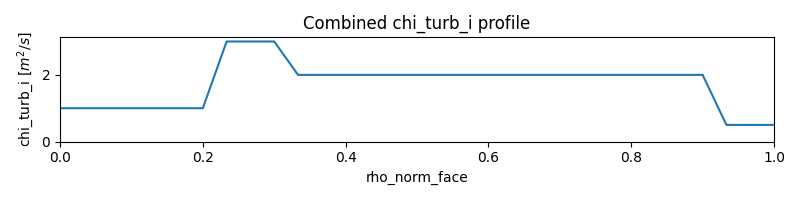
Note that in the region \([0, 0.2]\), only the first component is active, so chi_i = 1.0. In \((0.2, 0.3]\) the first two components are both active, leading to a combined value of chi_i = 3.0. In \((0.3, 0.9]\), only the second model is active (chi_i = 2.0), and in \((0.9, 1.0]\) only the pedestal transport model is active (chi_i = 0.5).

The code for generating the plot above is found in docs/scripts/combined_transport_example.py.

The next example shows how to apply a physics-based model (QLKNN) in the core, but enforcing specific transport coefficients in the edge region using a Constant model with OVERWRITE mode, effectively overriding the core model in that region. This is useful e.g. for L-mode modelling. This example is more powerful than using the outer_patch API, since we here have fine-grained control over each transport channel.

'transport': {
    'model_name': 'combined',
    'transport_models': [
        # Base model: QLKNN applied everywhere (default ADD)
        {
            'model_name': 'qlknn',
            'rho_max': 1.0,
        },
        # Edge overwrite: Sets D_e and V_e in the edge, ignoring QLKNN there.
        # Keeps chi_i/chi_e from QLKNN (because they are disabled here).
        {
            'model_name': 'constant',
            'rho_min': 0.9,
            'D_e': 0.5,
            'V_e': -1.0,
            'merge_mode': 'overwrite',
            'disable_chi_i': True,
            'disable_chi_e': True,
        },
    ],
  },

sources

Dictionary with nested dictionaries containing the configurable runtime parameters of all TORAX heat, particle, and current sources. The following runtime parameters are common to all sources, with defaults depending on the specific source. See Physics models For details on the source physics models.

Any source which is not explicitly included in the sources dict, is set to zero. To include a source with default options, the source dict should contain an empty dict. For example, for setting ei_exchange, with default options, as the only active source in sources, set:

'sources': {
    'ei_exchange': {},
}

The configurable runtime parameters of each source are as follows:

prescribed_values (time-varying-array [default = {0: {0: 0, 1: 0}}])

Time varying array of prescribed values for the source. Used if mode is 'PRESCRIBED'.

mode (str [default = ‘zero’])

Defines how the source values are computed. Currently the options are:

• 'ZERO'

  Source is set to zero.

• 'MODEL'

  Source values come from a model in code. Specific model selection where more than one model is available can be done by specifying a model_name. This is documented in the individual source sections.

• 'PRESCRIBED'

  Source values are arbitrarily prescribed by the user. The value is set by prescribed_values, and should be a tuple of values. Each value can contain the same data structures as Time-varying arrays. Note that these values are treated completely independently of each other so for sources with multiple time dimensions, the prescribed values should each contain all the information they need. For sources which affect multiple core profiles, look at the source’s affected_core_profiles property to see the order in which the prescribed values should be provided.

For example, to set ‘fusion_power’ to zero, e.g. for testing or sensitivity purposes, set:

'sources': {
    'fusion': {'mode': 'ZERO'},
}

To set ‘generic_current’ to a prescribed value based on a tuple of numpy arrays, e.g. as defined or loaded from a file in the preamble to the CONFIG dict within config module, set:

'sources': {
    'generic_current': {
        'mode': 'PRESCRIBED',
        'prescribed_values': ((times, rhon, current_profiles),),
    },

where the example times is a 1D numpy array of times, rhon is a 1D numpy array of normalized toroidal flux coordinates, and current_profiles is a 2D numpy array of the current profile at each time. These names are arbitrary, and can be set to anything convenient.

is_explicit (bool [default = False])

Defines whether the source is to be considered explicit or implicit. Explicit sources are calculated based on the simulation state at the beginning of a time step, or do not have any dependance on state. Implicit sources depend on updated states as the iterative solvers evolve the state through the course of a time step. If a source model is complex but evolves over slow timescales compared to the state, it may be beneficial to set it as explicit.

ei_exchange

Ion-electron heat exchange.

mode (str [default = ‘model’])

Qei_multiplier (float [default = 1.0])

Multiplication factor for ion-electron heat exchange term for testing purposes.

bremsstrahlung

Bremsstrahlung model from Wesson, with an optional correction for relativistic effects from Stott PPCF 2005.

mode (str [default = ‘model’])

use_relativistic_correction (bool [default = False])

cyclotron_radiation

Cyclotron radiation model from Albajar NF 2001 with a deposition profile from Artaud NF 2018.

mode (str [default = ‘model’])

wall_reflection_coeff (float [default = 0.9])

Machine-dependent dimensionless parameter corresponding to the fraction of cyclotron radiation reflected off the wall and reabsorbed by the plasma.

beta_min (float [default = 0.5])

beta_max (float [default = 8.0])

beta_grid_size (int [default = 32])

beta in this context is a variable in the temperature profile parameterization used in the Albajar model. The parameter is fit with simple grid search performed over the range [beta_min, beta_max], with beta_grid_size uniformly spaced steps. This parameter must be positive.

ecrh

Electron-cyclotron heating and current drive, based on the local efficiency model in Lin-Liu et al., 2003. Given an EC power density profile and efficiency profile, the model produces the corresponding EC-driven current density profile. The user has three options:

1. Provide an entire EC power density profile manually (via extra_prescribed_power_density).

2. Provide the parameters of a Gaussian EC deposition (via gaussian_width, gaussian_location, and P_total).

3. Any combination of the above.

By default, both the manual and Gaussian profiles are zero. The manual and Gaussian profiles are summed together to produce the final EC deposition profile.

mode (str [default = ‘model’])

extra_prescribed_power_density (time-varying-array [default = {0: {0: 0, 1: 0}}])

EC power density deposition profile, in units of \(W/m^3\).

gaussian_width (time-varying-scalar [default = 0.1])

Width of Gaussian EC power density deposition profile.

gaussian_location (time-varying-scalar [default = 0.0])

Location of Gaussian EC power density deposition profile on the normalized rho grid.

P_total (time-varying-scalar [default = 0.0])

Integral of the Gaussian EC power density profile, setting the total power.

current_drive_efficiency (time-varying-array [default = {0: {0: 0.2, 1: 0.2}}])

Dimensionless local efficiency profile for conversion of EC power to current.

fusion

DT fusion power from the Bosch-Hale parameterization. Uses the D and T fractions from the main_ion ion mixture.

mode (str [default = ‘model’])

gas_puff

Exponential based gas puff source. No first-principle-based model is yet implemented in TORAX.

mode (str [default = ‘model’])

puff_decay_length (time-varying-scalar [default = 0.05])

Gas puff decay length from edge in units of \(\hat{\rho}\).

S_total (time-varying-scalar [default = 1e22])

Total number of particle source in units of particles/s.

generic_current

Generic external current profile, parameterized as a Gaussian.

mode (str [default = ‘model’])

gaussian_location (time-varying-scalar [default = 0.4])

Gaussian center of current profile in units of \(\hat{\rho}\).

gaussian_width (time-varying-scalar [default = 0.05])

Gaussian width of current profile in units of \(\hat{\rho}\).

I_generic (time-varying-scalar [default = 3.0e6])

Total current in A. Only used if use_absolute_current==True.

fraction_of_total_current (time-varying-scalar [default = 0.2])

Sets total generic_current to be a fraction fraction_of_total_current of the total plasma current. Only used if use_absolute_current==False.

use_absolute_current (bool [default = False])

Toggles relative vs absolute external current setting.

generic_heat

A utility source module that allows for a time-dependent Gaussian ion and electron heat source.

mode (str [default = ‘model’])

gaussian_location (time-varying-scalar [default = 0.0])

Gaussian center of source profile in units of \(\hat{\rho}\).

gaussian_width (time-varying-scalar [default = 0.25])

Gaussian width of source profile in units of \(\hat{\rho}\).

P_total (time-varying-scalar [default = 120e6])

Total source power in W. High default based on total ITER power including alphas.

electron_heat_fraction (time-varying-scalar [default = 0.66666])

Electron heating fraction.

absorption_fraction (time-varying-scalar [default = 0.0])

Fraction of input power that is absorbed by the plasma.

generic_particle

Time-dependent Gaussian particle source. No first-principle-based model is yet implemented in TORAX.

mode (str [default = ‘model’])

deposition_location (time-varying-scalar [default = 0.0])

Gaussian center of source profile in units of \(\hat{\rho}\).

particle_width (time-varying-scalar [default = 0.25])

Gaussian width of source profile in units of \(\hat{\rho}\).

S_total (time-varying-scalar [default = 1e22])

Total particle source in units of particles/s.

icrh

Ion cyclotron resonance heating (ICRH) source. Two model implementations are available, selected via the model_name discriminator.

mode (str [default = ‘model’])

P_total (time-varying-scalar [default = 10e6])

Total injected source power in W.

absorption_fraction (time-varying-scalar [default = 1.0])

Fraction of P_total absorbed by the plasma.

model_name (str)

Selects the ICRH model. Available options:

• 'toric_nn' (default)

  Surrogate model of the TORIC ICRH spectrum solver simulation https://meetings.aps.org/Meeting/DPP24/Session/NP12.106. This source is currently SPARC specific.

  Weights and configuration for the surrogate model are needed to use this source. By default these are expected to be found under '~/toric_surrogate/TORIC_MLP_v1/toricnn.json'. To use a different file path an alternative path can be provided using the TORIC_NN_MODEL_PATH environment variable which should point to a compatible JSON file.

  model_path (str | None [default = None])

  Path to the JSON file containing the weights and configuration for the surrogate model. If None, the default path '~/toric_surrogate/TORIC_MLP_v1/toricnn.json' is used.

  wall_inner (float [default = 1.24])

  Inner radial location of first wall at plasma midplane level [m].

  wall_outer (float [default = 2.43])

  Outer radial location of first wall at plasma midplane level [m].

  frequency (time-varying-scalar [default = 120e6])

  ICRF wave frequency in Hz.

  minority_concentration (time-varying-scalar [default = 0.03])

  Helium-3 minority fractional concentration relative to the electron density. This is a deprecated legacy option, used only when minority_species is not specified. It is recommended to instead set minority_species to ‘He3’ and use the plasma composition to set the minority concentration.

  minority_species (str | None [default = None])

  Symbol of the minority species (e.g. ‘He3’). If specified, the minority concentration is automatically extracted from the plasma composition. Presently, only ‘He3’ is supported.

• 'scaled_profile'

  Prescribed-profile model with magnetic-field-dependent resonance shifting. Adapts reference heating profiles to different magnetic field operating points and normalises them to the target power. See Physics models for detailed physics description.

  heat_profile_ion (time-varying-array [default = {0: {0: 0, 1: 0}}])

  Reference ion heating power density shape [W/m³], provided on the normalised radius grid. The shape is rescaled during normalisation; only the relative profile matters.

  heat_profile_electron (time-varying-array [default = {0: {0: 0, 1: 0}}])

  Reference electron heating power density shape [W/m³], provided on the normalised radius grid.

  reference_B0 (time-varying-scalar [default = 12.2])

  Vacuum toroidal magnetic field at which the reference profiles were computed [T].

  Example:

  'sources': {
      'icrh': {
          'model_name': 'scaled_profile',
          'P_total': 25e6,
          'absorption_fraction': 0.9,
          'heat_profile_ion': {0: {0.0: 0, 0.3: 1.0, 0.6: 0.2, 1.0: 0}},
          'heat_profile_electron': {0: {0.0: 0, 0.35: 0.8, 0.65: 0.1, 1.0: 0}},
          'reference_B0': 12.2,
      },
  }
  

See Physics models for more detail.

impurity_radiation

Various models for impurity radiation. Runtime params for each available model are listed separately

mode (str [default = ‘model’])

model_name (str [default = ‘mavrin_fit’])

The following models are available:

• 'mavrin_fit'

  Polynomial fits to ADAS data from Mavrin, 2018.

  radiation_multiplier (float [default = 1.0]). Multiplication factor for radiation term for testing sensitivities.

• 'P_in_scaled_flat_profile'

  Sets impurity radiation to be a constant fraction of the total external input power.

  fraction_P_heating (float [default = 1.0]). Fraction of total external input heating power to use for impurity radiation.

ohmic

Ohmic power.

mode (str [default = ‘model’])

pellet

Time-dependent Gaussian pellet source. No first-principle-based model is yet implemented in TORAX.

mode (str [default = ‘model’])

pellet_deposition_location (time-varying-scalar [default = 0.85])

Gaussian center of source profile in units of \(\hat{\rho}\).

pellet_width (time-varying-scalar [default = 0.1])

Gaussian width of source profile in units of \(\hat{\rho}\).

S_total (time-varying-scalar [default = 2e22])

Total particle source in units of particles/s

mhd

Configuration for MHD models. Currently only the sawtooth model is implemented. If the mhd key or the nested sawtooth key is absent or set to None, the sawtooth model will be disabled.

sawtooth

model_name (str [default = ‘simple’])

Currently only ‘simple’ is supported.

simple trigger model parameters:

• s_critical (time-varying-scalar [default = 0.1]) The critical magnetic shear value at the q=1 surface. A crash is triggered only if the shear exceeds this value.

• minimum_radius (time-varying-scalar [default = 0.05]) The minimum normalized radius (\(\hat{\rho}\)) of the q=1 surface required to trigger a crash.

model_name (str [default = ‘simple’])

Currently only ‘simple’ is supported.

simple redistribution model parameters:

• flattening_factor (time-varying-scalar [default = 1.01]): Factor determining the degree of flattening inside the q=1 surface.

• mixing_radius_multiplier (time-varying-scalar [default = 1.1]): Multiplier applied to \(\hat{\rho}_{q=1}\) to determine the mixing radius \(\hat{\rho}_{mix}\).

crash_step_duration (float [default = 1e-5]):

Duration of a sawtooth crash step in seconds. This is how much the solver time will be bumped forward during a crash. It is important that this is is small enough to satisfy the assumption of timescale separation between the sawtooth crash and the transport timescale, otherwise issues may arise regarding conservation properties.

solver

Select and configure the Solver object, which evolves the PDE system by one timestep. See TORAX solver details for further details. The dictionary consists of keys common to all solvers. Additional fields for parameters pertaining to a specific solver are defined in the relevant section below.

solver_type (str [default = ‘linear’])

Selected PDE solver algorithm. The current options are:

• 'linear'

  Linear solver where PDE coefficients are set at fixed values of the state. An approximation of the nonlinear solution is optionally carried out with a predictor-corrector method, i.e. fixed point iteration of the PDE coefficients.

• 'newton_raphson'

  Nonlinear solver using the Newton-Raphson iterative algorithm, with backtracking line search, and timestep backtracking, for increased robustness.

• 'optimizer'

  Nonlinear solver using the jaxopt library.

theta_implicit (float [default = 1.0])

theta value in the theta method of time discretization. 0 = explicit, 1 = fully implicit, 0.5 = Crank-Nicolson.

use_predictor_corrector (bool [default = True])

Enables use_predictor_corrector iterations with the linear solver.

n_corrector_steps (int [default = 10])

Number of corrector steps for the predictor-corrector linear solver. 0 means a pure linear solve with no corrector steps. Must be a positive integer.

atol (float | None [default = None])

Absolute tolerance for fixed-point iterations in the predictor-corrector solver. If specified, iterations can exit early when the normalized residual falls below this threshold.

rtol (float | None [default = None])

Relative tolerance for fixed-point iterations in the predictor-corrector solver. If specified, iterations can exit early when the normalized residual falls below this fraction of the initial residual.

fixed_point_termination_criterion (str [default = ‘max_iterations’])

Termination criterion for the fixed-point iterations in the predictor-corrector solver. Must be either ‘tolerance’ (exit when tolerances are met) or ‘max_iterations’ (always run for the specified number of iterations).

use_pereverzev (bool [default = False])

Use Pereverzev-Corrigan terms in the heat and particle flux when using the linear solver. Critical for stable calculation of stiff transport, at the cost of introducing non-physical lag during transient. Also used for the linear_step initial guess mode in the nonlinear solvers.

chi_pereverzev (float [default = 30.0])

Large heat conductivity used for the Pereverzev-Corrigan term.

D_pereverzev (float [default = 15.0])

Large particle diffusion used for the Pereverzev-Corrigan term.

implicit_solver_type (str [default = ‘THOMAS’])

Selects the algorithm used to solve the block-tridiagonal linear system that arises at each implicit time step. The available options are:

• 'THOMAS'

  The Thomas algorithm (block LU factorization), which solves the system in linear complexity in the number of grid cells by exploiting the tridiagonal sparsity structure. This is the recommended default for most simulations.

• 'DENSE'

  Converts the block-tridiagonal system to a dense matrix and solves it with a general-purpose linear solver. This is primarily useful for debugging, validation or small systems, as it does not exploit sparsity and scales as cubicly with the number of grid cells.

linear

No extra parameters are defined for the linear solver.

newton_raphson

log_iterations (bool [default = False])

If True, logs information about the internal state of the Newton-Raphson solver. For the first iteration, this contains the initial residual value and time-step size. For subsequent iterations, this contains the iteration step number, the current value of the residual, and the current value of tau, which is the relative reduction in Newton step size compared to the original Newton step size. If the solver does not converge, then these inner iterations will restart at a smaller timestep size if adaptive_dt=True in the numerics config dict.

initial_guess_mode (str [default = ‘linear_step’])

Sets the approach taken for the initial guess into the Newton-Raphson solver for the first iteration. Two options are available:

• x_old

  Use the state at the beginning of the timestep.

• linear_step

  Use the linear solver to obtain an initial guess to warm-start the nonlinear solver. If used, is recommended to do so with the use_predictor_corrector solver and several corrector steps. It is also strongly recommended to use_pereverzev=True if a stiff transport model like qlknn is used.

residual_tol (float [default = 1e-5])

PDE residual magnitude tolerance for successfully exiting the iterative solver.

residual_coarse_tol (float [default = 1e-2])

If the solver hits an exit criterion due to small steps or many iterations, but the residual is still below coarse_tol, then the step is allowed to successfully pass, and a warning is passed to the user.

n_max_iterations (int [default = 30])

Maximum number of allowed Newton iterations. If the number of iterations surpasses maxiter, then the solver will exit in an unconverged state. The step will still be accepted if residual < coarse_tol, otherwise dt backtracking will take place if enabled.

delta_reduction_factor (float [default = 0.5])

Reduction of Newton iteration step size in the backtracking line search. If in a given iteration, the new state is unphysical (e.g. negative temperatures) or the residual increases in magnitude, then a smaller step will be iteratively taken until the above conditions are met.

tau_min (float [default = 0.01])

tau is the relative reduction in step size: delta/delta_original, following backtracking line search, where delta_original is the step in state \(x\) that minimizes the linearized PDE system. If following some iterations, tau < tau_min, then the solver will exit in an unconverged state. The step will still be accepted if residual < coarse_tol, otherwise dt backtracking will take place if enabled.

optimizer

initial_guess_mode (str [default = ‘linear_step’])

Sets the approach taken for the initial guess into the Newton-Raphson solver for the first iteration. Two options are available:

• x_old

  Use the state at the beginning of the timestep.

• linear_step

  Use the linear solver to obtain an initial guess to warm-start the nonlinear solver. If used, is recommended to do so with the use_predictor_corrector solver and several corrector steps. It is also strongly recommended to use_pereverzev=True if a stiff transport model like qlknn is used.

loss_tol (float [default = 1e-10])

PDE loss magnitude tolerance for successfully exiting the iterative solver. Note: the default tolerance here is smaller than the default tolerance for the Newton-Raphson solver because it’s a tolerance on the loss (square of the residual).

n_max_iterations (int [default = 100])

Maximum number of allowed optimizer iterations.

time_step_calculator

calculator_type (str [default = ‘chi’])

The name of the time_step_calculator, a method which calculates dt at every timestep. Three methods are currently available:

• 'fixed'

  dt is equal to fixed_dt defined in numerics. If the Newton-Raphson solver is being used and adaptive_dt==True in the numerics config dict, then in practice some steps may have lower dt if the solver needed to backtrack.

• 'chi'

  adaptive dt method, where dt is a multiple of a base dt inspired by the explicit stability limit for parabolic PDEs: \(dt_{base}=\frac{dx^2}{2\chi}\), where \(dx\) is the grid resolution and \(\chi=max(\chi_i, \chi_e)\). dt=chi_timestep_prefactor * dt_base, where chi_timestep_prefactor is defined in numerics, and can be significantly larger than unity for implicit solvers. Scaling the timestep to be \(\propto \chi\) helps protect against traversing through fast transients, if there is a desire for them to be fully resolved.

• 'from_previous_dt'

  dt is equal to the previous time step duration multiplied by the dt_reduction_factor defined in numerics. This can speed

  up simulations that take many dt reduction steps, as the dt is initialized to a smaller value, rather than starting from max_dt every time. It can also speed up simulations where a small dt is required for a short section, but then a larger dt is be appropriate for the remainder of the simulation.

tolerance (float [default = 1e-7])

The tolerance within the final time for which the simulation will be considered done.

neoclassical

bootstrap_current

model_name (str [default = ‘sauter’])

The name of the model to use. If not provided, the default is to use the Sauter model with default values. One of sauter or zeros is supported.

If the sauter model is used, the following parameters can be set:

bootstrap_multiplier (float [default = 1.0])

Multiplier for the bootstrap current.

conductivity

model_name (str [default = ‘sauter’])

The name of the Sauter model to use. If not provided, the default is to use the Sauter model with default values.

transport

model_name (str [default = ‘zeros’])

The name of the neoclassical transport model. The following models are supported:

• 'zeros' Sets all neoclassical transport coefficients to zero.

• 'angioni_sauter' The Angioni-Sauter neoclassical transport model from C. Angioni and O. Sauter, Phys. Plasmas 7, 1224 (2000). This is the default model. This model does not have any additional configurable parameters.

chi_min (float [default = 0.0])

Lower allowed bound for neoclassical heat conductivities \(\chi_\mathrm{neo}\), in units of \(m^2/s\).

chi_max (float [default = 100.0])

Upper allowed bound for neoclassical heat conductivities \(\chi_\mathrm{neo}\), in units of \(m^2/s\).

D_e_min (float [default = 0.0])

Lower allowed bound for neoclassical particle diffusivity \(D_\mathrm{neo}\), in units of \(m^2/s\).

D_e_max (float [default = 100.0])

Upper allowed bound for neoclassical particle conductivity \(D_\mathrm{neo}\), in units of \(m^2/s\).

V_e_min (float [default = -50.0])

Lower allowed bound for neoclassical particle convection terms \(V_\mathrm{neo}\) and \(V_\mathrm{neo, ware}\) in units of \(m^2/s\). Note that clipping to the desired range will be applied to \(V_\mathrm{neo}\) and \(V_\mathrm{neo, ware}\) separately.

V_e_max (float [default = 50.0])

Upper allowed bound for neoclassical particle convection terms \(V_\mathrm{neo}\) and \(V_\mathrm{neo, ware}\) in units of \(m^2/s\). Note that clipping to the desired range will be applied to \(V_\mathrm{neo}\) and \(V_\mathrm{neo, ware}\) separately.

poloidal_velocity_multiplier (float [default = 1.0])

Multiplier for the poloidal velocity.

restart

If this optional entry is supplied in the config, TORAX will be run starting from the selected state in a previous simulation. This can be used to resume a completed simulation.

If the requested restart time is not exactly available in the state file, the simulation will restart from the closest available time. A warning will be logged in this case.

filename (PathLike)

Path to an existing TORAX output file (netCDF format).

time (float)

Time in output file to load as the new initial state.

do_restart (bool)

If True, perform the restart from the selected state. If False, disable the restart and run the simulation as normal.

stitch (bool)

If True, concatenate the old and new simulation histories in the resulting output file. If False, output file will only contain the new history.

For example, following a simulation in which a state file is saved to /path/to/torax_state_file.nc, a new simulation can be started from the old state at t=10 by adding the following to the config:

'restart': {
    'filename': '/path/to/torax_state_file.nc',
    'time': 10,
    'do_restart': True,
    'stitch': True,
}

The resulting simulation will recreate the state from t=10 in the previous simulation, and then run forwards from that point in time. For all subsequent steps the runtime parameters will be constructed using the runtime parameter configuration provided in the new config (from t=10 onwards).

If the requested restart time is not exactly available in the state file, the simulation will restart from the closest available time. A warning will be logged in this case.

Some potential use cases for this feature include:

• Restarting a simulation that was healthy up to a certain time and then failed. After fixing the cause of the failure, a new simulation can be run from the last healthy point.

• Performing uncertainty quantification by sweeping a set of configs starting from the same initial plasma state. After performing an initial simulation, the restart option could be used to run a set of configs with modified parameters to evaluate the impact of their variation.

Additional Notes

What triggers a recompilation?

Most config options can be changed without recompiling the simulation code.

Some define the fundamental structure of the simulation and require JAX recompilation if changed. Examples include the number of grid points or the choice of transport model. A partial list is provided below.

• CONFIG['geometry']['nrho']

• CONFIG['numerics']['evolve_ion_heat']

• CONFIG['numerics']['evolve_electron_heat']

• CONFIG['numerics']['evolve_current']

• CONFIG['numerics']['evolve_density']

• CONFIG['transport']['model_name']

• CONFIG['solver']['solver_type']

• CONFIG['time_step_calculator']['calculator_type']

• CONFIG['sources']['source_name']['is_explicit']

• CONFIG['sources']['source_name']['mode']

In the future we aim to provide more transparency at the config level for which configuration options recompilation is required.

Using IMAS input data

Loading Geometry

The geometry in TORAX can be constructed from IMAS equilibium IDSs. The specific arguments to load an equilibrium IDS with TORAX are specified in geometry.

There are three main methods to load IMAS equilibrium:

• Using IMAS netCDF file (imas_filepath). This is the main method as it does not require the optional dependency to imas-core. The path of the file can then be provided in the config to run TORAX with this geometry.

• Using IMAS uri (imas_uri). This method does require the imas-core dependency. It loads the equilibrium data from the given IDS with a backend of choice.

• Providing the equilibium IDS on the fly (equilibrium_object). Using this method the IDS can be provided externally or pre-loaded.

Loading Profiles

Profiles in TORAX can be read from any IMAS core_profiles or plasma_profiles IDS saved in Data Dictionary version 4.0.0 or newer. If the IDS is stored in an IMAS db or in a netCDF file it can be loaded using the loader function load_imas_data from |imas_loader|. It can then be loaded programatically in the CONFIG by constructing a nested dictionary with the profile_conditions_from_imas and plasma_composition_from_imas functions from |core_profiles_input_imas|. The functions returns a dictionary whose structure fits the schema of profile_conditions or plasma_composition and can be programatically loaded into a CONFIG with standard dictionary manipulation.

An example on how to inject the IMAS conditions into the config can be found in the test file imas_tools/input/tests/core_profiles_test.py. It is possible to directly input all of profile_conditions from an IDS into the config, or to only load specific values of it. It is also possible to combine profiles from different IDSs and their time slices can be shifted to correct offsets between different IDSs or to match the config t_initial.

Config example

An example configuration dict, corresponding to a non-rigorous demonstration mock-up of a time-dependent ITER hybrid scenario rampup (presently with a fixed CHEASE geometry), is shown below. The configuration file is also available in torax/examples/iterhybrid_rampup.py.

CONFIG = {
    'plasma_composition': {
        'main_ion': {'D': 0.5, 'T': 0.5},
        'impurity': 'Ne',
        'Z_eff': 1.6,
    },
    'profile_conditions': {
        'Ip': {0: 3e6, 80: 10.5e6},
        # initial condition ion temperature for r=0 and r=a_minor
        'T_i': {0.0: {0.0: 6.0, 1.0: 0.1}},
        'T_i_right_bc': 0.1,  # boundary condition ion temp for r=a_minor
        # initial condition electron temperature between r=0 and r=a_minor
        'T_e': {0.0: {0.0: 6.0, 1.0: 0.1}},
        'T_e_right_bc': 0.1,  # boundary condition electron temp for r=a_minor
        'n_e_right_bc_is_fGW': True,
        'n_e_right_bc': {0: 0.1, 80: 0.3},
        'n_e_nbar_is_fGW': True,
        'nbar': 1,
        'n_e': {0: {0.0: 1.5, 1.0: 1.0}},  # Initial electron density profile
    },
    'numerics': {
        't_final': 80,
        'fixed_dt': 2,
        'evolve_ion_heat': True,
        'evolve_electron_heat': True,
        'evolve_current': True,
        'evolve_density': True,
        'dt_reduction_factor': 3,
        'adaptive_T_source_prefactor': 1.0e10,
        'adaptive_n_source_prefactor': 1.0e8,
    },
    'geometry': {
        'geometry_type': 'chease',
        'geometry_file': 'iterhybrid.mat2cols',
        'Ip_from_parameters': True,
        'R_major': 6.2,
        'a_minor': 2.0,
        'B_0': 5.3,
    },
    'neoclassical': {
        'bootstrap_current': {
            'bootstrap_multiplier': 1.0,
        },
    },
    'sources': {
        'generic_current': {
            'fraction_of_total_current': 0.15,
            'gaussian_width': 0.075,
            'gaussian_location': 0.36,
        },
        'pellet': {
            'S_total': 0.0e22,
            'pellet_width': 0.1,
            'pellet_deposition_location': 0.85,
        },
        'generic_heat': {
            'gaussian_location': 0.12741589640723575,
            'gaussian_width': 0.07280908366127758,
            # total heating (with a rough assumption of radiation reduction)
            'P_total': 20.0e6,
            'electron_heat_fraction': 1.0,
        },
        'fusion': {},
        'ei_exchange': {},
    },
    'transport': {
        'model_name': 'qlknn',
        'apply_inner_patch': True,
        'D_e_inner': 0.25,
        'V_e_inner': 0.0,
        'chi_i_inner': 1.5,
        'chi_e_inner': 1.5,
        'rho_inner': 0.3,
        'apply_outer_patch': True,
        'D_e_outer': 0.1,
        'V_e_outer': 0.0,
        'chi_i_outer': 2.0,
        'chi_e_outer': 2.0,
        'rho_outer': 0.9,
        'chi_min': 0.05,
        'chi_max': 100,
        'D_e_min': 0.05,
        'D_e_max': 50,
        'V_e_min': -10,
        'V_e_max': 10,
        'smoothing_width': 0.1,
        'DV_effective': True,
        'avoid_big_negative_s': True,
        'An_min': 0.05,
        'ITG_flux_ratio_correction': 1,
    },
    'pedestal': {
        'model_name': 'set_T_ped_n_ped',
        'set_pedestal': True,
        'T_i_ped': 1.0,
        'T_e_ped': 1.0,
        'n_e_ped': {0: 0.3, 80: 0.7},
        'rho_norm_ped_top': 0.95,
        'n_e_ped_is_fGW': True,
    },
    'solver': {
        'solver_type': 'newton_raphson',
        'use_predictor_corrector': True,
        'n_corrector_steps': 10,
        'chi_pereverzev': 30,
        'D_pereverzev': 15,
        'use_pereverzev': True,
        'log_iterations': False,
    },
    'time_step_calculator': {
        'calculator_type': 'fixed',
    },
}